Cosmological parameters and the evolution of the universe

Introduction

Modern cosmology begins with Hubble (1929), who established the linear relation between recession velocity and distance. This work approaches that relation from three complementary angles:

1. H₀ is estimated by replicating the analysis of the 24 original nebulae and compared with the current values from Planck (Planck Collaboration et al., 2020) and SH0ES (Riess et al., 2022), discussing the origin of the discrepancies.
2. The Friedmann equations are applied to a universe dominated by a single component with equation of state w = 1 (stiff matter), and the scale factor, the Hubble parameter, the deceleration, the age and the size of the universe are derived, as well as the emission time and the distance of a source at z = 2.
3. Recombination is studied with the Saha equation (η = 10⁻⁹; X = 0.1, 0.5 and 0.9), together with the decoupling of the cosmic microwave background photons, assessing the influence of the value of H₀ adopted.

1. Calculation of the Hubble constant

In 1929 Edwin Hubble published observational evidence that extragalactic nebulae (now called galaxies) are receding from us with a velocity proportional to their distance (Hubble, 1929). To show this, he built a diagram of radial velocity against distance with 24 objects whose distances could be estimated independently. The method consists of:

1. Measuring the radial velocity v of each nebula from the redshift of its spectral lines, applying the Doppler effect.
2. Estimating the distance r with luminosity indicators: Cepheid variables, novae, blue stars in emission nebulae and the upper limit of absolute luminosity of the brightest resolved stars.
3. Plotting v against r and looking for a linear correlation of the form v = H₀ · r.
4. Fitting by least squares the slope H₀ (the Hubble constant), which represents the expansion rate of the universe.

Why are the variables r and v used?

The distance r (in units of 10⁶ parsecs, or Mpc) is the independent variable because it represents the spatial separation between the observer and the nebula. In an expanding universe described by the Friedmann–Lemaître–Robertson–Walker metric (Carroll, 2004), the distance between comoving objects grows with the scale factor a(t). Measuring r makes it possible to quantify how much space has expanded between us and the object.

The radial velocity v (in km/s) is the dependent variable because it is the observable consequence of that expansion. The redshift of the spectral lines directly gives the radial component of the recession velocity. If the universe expands uniformly, v must be proportional to r: more distant objects recede faster because there is more space between them expanding at the same time.

The linear relation v = H₀ · r is a direct prediction of a homogeneous, isotropic, expanding universe. The slope H₀ has units of km/s/Mpc (equivalent to a frequency, s⁻¹), and its inverse, 1/H₀, gives a first estimate of the time elapsed since the start of the expansion (the age of the universe to a first approximation).

The original data of Table 1 of Hubble (1929) are reproduced below; the method described is applied to them:

• m_s: photographic magnitude of the brightest stars involved.
• r: distance in units of 10⁶ parsecs.
• v: measured velocity in km/s.
• m_t: Holetschek’s visual magnitude as corrected by Hopmann.
• M_t: total visual absolute magnitude (calculated from m_t and r).

Object	ms	r (Mpc)	v (km/s)	mt	Mt
S. Mag.	—	0.032	170	1.5	−16.0
L. Mag.	—	0.034	290	0.5	−17.2
NGC 6822	—	0.214	−130	9.0	−12.7
NGC 598	—	0.263	−70	7.0	−15.1
NGC 221	—	0.275	−185	8.8	−13.4
NGC 224	—	0.275	−220	5.0	−17.2
NGC 5457	17.0	0.450	200	9.9	−13.3
NGC 4736	17.3	0.500	290	8.4	−15.1
NGC 5194	17.3	0.500	270	7.4	−16.1
NGC 4449	17.8	0.630	200	9.5	−14.5
NGC 4214	18.3	0.800	300	11.3	−13.2
NGC 3031	18.5	0.900	−30	8.3	−16.4
NGC 3627	18.5	0.900	650	9.1	−15.7
NGC 4826	18.5	0.900	150	9.0	−15.7
NGC 5236	18.5	0.900	500	10.4	−14.4
NGC 1068	18.7	1.000	920	9.1	−15.9
NGC 5055	19.0	1.100	450	9.6	−15.6
NGC 7331	19.0	1.100	500	10.4	−14.8
NGC 4258	19.5	1.400	500	8.7	−17.0
NGC 4151	20.0	1.700	960	12.0	−14.2
NGC 4382	—	2.000	500	10.0	−16.5
NGC 4472	—	2.000	850	8.8	−17.7
NGC 4486	—	2.000	800	9.7	−16.8
NGC 4649	—	2.000	1090	9.5	−17.0

Table 1. Nebulae whose distances were estimated from their constituent stars or from the mean luminosities of a cluster (Hubble, 1929).

With the original data presented, the next step is to apply points 3 and 4 of the method: plot the radial velocity v against the distance r and obtain the Hubble constant as the slope of the best-fit line. Two lines are overlaid on the data (Figure 1): the red one, corresponding to the free linear fit, and the blue one, corresponding to the fit forced through the origin. At first sight both are similar, but the difference between their slopes and the position of the intercept contain relevant cosmological information.

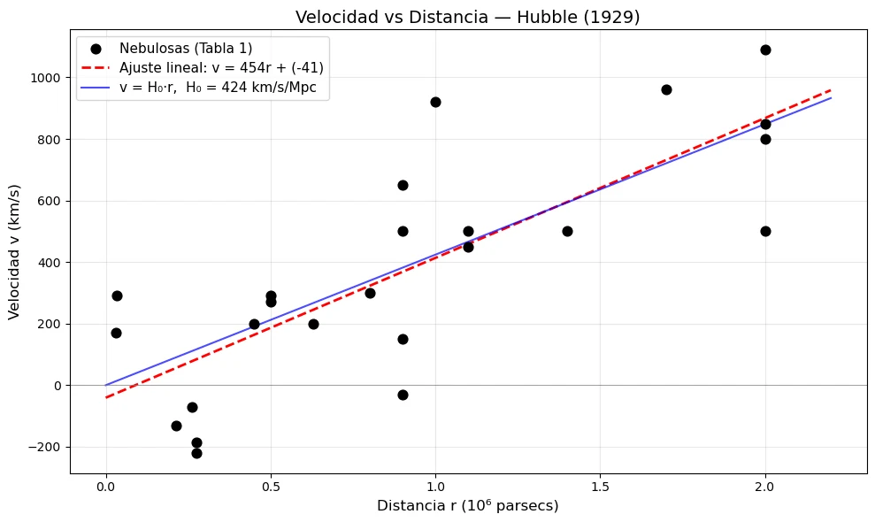
Free linear fit (red line): v = H₀ · r + v₀. This is a least-squares linear regression in which both the slope H₀ and the intercept v₀ are free parameters. The intercept v₀ ≠ 0 absorbs systematic effects such as the peculiar motion of the Sun with respect to the cosmic rest frame, errors in the distances of the nearest objects and the peculiar velocities of individual nebulae. Statistically, this fit minimises the sum of squared residuals without imposing physical constraints.

Fit forced through the origin (blue line): v = H₀ · r. Here the physical condition is imposed that, at zero distance, the recession velocity must vanish (v₀ = 0). This directly reflects Hubble’s law: the expansion of the universe implies that the recession velocity is proportional to distance, with no constant term. The value of H₀ obtained is the Hubble constant.

Which is more physically correct? The blue line has greater cosmological meaning, because it is exactly what Hubble’s law predicts, v = H₀ r. The difference between the two lines reveals the size of the peculiar velocities and of the systematic errors in the data. In a perfectly homogeneous and isotropic universe both lines would coincide; the discrepancy indicates that nearby objects have significant motions of their own with respect to the Hubble flow.

Applying both procedures to the data in Table 1 gives the results in Table 2.

Fit	Parameter	Value	Units
Free linear (v = H₀·r + v₀)	Slope H₀	454.2	km/s/Mpc
	Intercept v₀	−40.8	km/s
	R²	0.6235	—
	p-value	4.48 × 10⁻⁶	—
Forced through the origin (v = H₀·r)	H₀	423.9 ± 75.2	km/s/Mpc

Table 2. Results of the linear regressions on the data in Table 1.

It should be noted that Hubble himself (1929), using a method of group averages on the same objects, obtained a value close to 500 km/s/Mpc; the difference from the least-squares fit of this work is due to that different methodology. In any case, both values are radically different from modern cosmological measurements (between 67 and 73 km/s/Mpc), a discrepancy of a factor of 6 to 7 that deserves a detailed analysis.

Why does Hubble’s H₀ (1929) not match current values?

The value obtained by Hubble in 1929 was H₀ ≈ 500 km/s/Mpc, whereas modern measurements converge around the following values:

• Planck (CMB, 2018): H₀ = 67.4 ± 0.5 km/s/Mpc, from the analysis of the cosmic microwave background (Planck Collaboration et al., 2020).
• SH0ES / Hubble Space Telescope (Cepheids + SNe Ia): H₀ = 73.04 ± 1.04 km/s/Mpc, from the calibration of the local distance scale with Cepheids and type Ia supernovae (Riess et al., 2022).
• Hubble (1929): H₀ ≈ 500 km/s/Mpc, a value that in this work, with a least-squares fit forced through the origin, is recalculated as H₀ ≈ 424 km/s/Mpc.

Hubble overestimated H₀ by a factor of 6 to 7 (7 with his value of 500 km/s/Mpc; 6 with the recalculated 424). The reasons are many and are now well understood:

1. Error in the distance calibration (cosmic distance scale). Hubble used the period–luminosity relation of Cepheids calibrated by Shapley (1918), which contained a fundamental systematic error: it did not distinguish between classical Cepheids (population I) and W Virginis variables (population II). W Virginis stars are ~1.5 magnitudes fainter for the same period, which caused distances to be underestimated by a factor of ~2. Walter Baade corrected this in 1952 and immediately doubled the distance scale.
2. Confusion between stars and HII regions. In the most distant nebulae, what Hubble identified as “the brightest stars” were in fact unresolved HII regions (clouds of ionised hydrogen), much more luminous than individual stars (Sandage, 1958). This led to the distances of the most distant objects in the sample being underestimated.
3. Limited sample and selection biases. The sample contained only 24 objects, all within a radius of ~2 Mpc. At such short distances, the peculiar velocities of galaxies (local gravitational, not cosmological, motions) are comparable to or larger than the recession velocity due to expansion (Strauss and Willick, 1995). This introduces a huge scatter and biases the slope. Modern measurements use objects at hundreds or thousands of Mpc, where peculiar velocities are negligible compared with the Hubble flow.
4. Uncorrected interstellar absorption. In 1929, extinction by dust was not well known; Trumpler (1930) would quantify it for the first time the year after Hubble’s work. The apparent magnitudes were not corrected for absorption, which affected the distance estimates based on luminosity.
5. Zero point of the period–luminosity relation. The absolute zero point of the Cepheid P–L relation depended on calibrations with Galactic star clusters whose distances were imprecise. Each improvement in parallaxes, from Hipparcos (Perryman et al., 1997) to Gaia (Gaia Collaboration et al., 2023), has refined this zero point.

Today there is a discrepancy of ~5σ between the value of H₀ measured locally (SH0ES: ~73 km/s/Mpc; Riess et al., 2022) and the one inferred from the CMB (Planck: ~67 km/s/Mpc; Planck Collaboration et al., 2020). This Hubble tension is an open problem in cosmology and could point to new physics beyond the standard ΛCDM model or to systematic errors not yet identified in one of the methods (Verde et al., 2019; Di Valentino et al., 2021). The first measurements with the James Webb Space Telescope have revived the debate: the CCHP programme obtains H₀ ≈ 70.4 km/s/Mpc with the TRGB method, compatible with both ends (Freedman et al., 2025), while the SH0ES team confirms its Cepheid calibration with JWST (≈ 73 km/s/Mpc; Riess et al., 2024). The tension remains open, but both new physics and systematic errors are now being debated.

2. Universe dominated by a single component with w = 1

In cosmology, solving the Friedmann equations simultaneously with all the components of the universe (matter, radiation and dark energy) does not admit a closed analytical solution and requires numerical integration. A common teaching strategy is therefore to consider an idealised universe dominated by a single component, which yields closed expressions for the cosmological observables and helps to understand the individual role of each parameter (Ryden, 2017).

This section addresses the case of a fluid with equation of state w = 1, known as stiff matter, in which the pressure equals the energy density. Although no known component satisfies exactly this equation of state in today’s universe, scenarios dominated by stiff matter have been proposed for extremely early epochs of the universe, even before the radiation era (Zel’dovich, 1962).

A flat universe dominated by a single component with w = 1 is considered, with a₀ = 1 (present scale factor normalised to unity). The results are compared for:

• H₀,Hubble 1929 ≈ 424 km/s/Mpc, the value obtained from the fit through the origin in the previous section.
• H₀ = 70 km/s/Mpc, a modern reference value.

The Friedmann equations (Friedmann, 1922) are derived by applying the field equations of general relativity to a spatially homogeneous and isotropic metric (FLRW), under the cosmological principle that the properties of the universe are the same at every point and in every direction on large scales (Carroll, 2004). Only two equations of this system are needed: the first relates the expansion rate H to the total energy density ρ, and the second, derived from the first together with energy conservation, describes how ρ evolves with the scale factor. For a perfect fluid with a constant equation of state P = w · ρc², this evolution takes the general form developed below (Kolb and Turner, 1990).

Friedmann equations for a single component

The first Friedmann equation results from applying general relativity to a homogeneous, isotropic, flat universe (Friedmann, 1922):

H² = (ȧ / a)² = (8πG / 3) · ρ

For a perfect fluid with equation of state P = wρc², the energy density evolves as:

ρ(a) = ρ₀ · a^−3(1+w)

Returning to the first Friedmann equation and substituting ρ(a) with w = 1:

H² = (8πG / 3) · ρ₀ · a⁻⁶

Applying the present-day normalisation, that is, evaluating the equation at a = a₀ = 1, where H = H₀:

H₀² = (8πG / 3) · ρ₀

1. Scale factor a(t). Substituting H₀ into the previous equation gives H² = H₀² a⁻⁶. Taking the square root and solving for ȧ:

ȧ / a = H₀ a⁻³ ⟹ ȧ = H₀ a⁻²

Separating variables, a² da = H₀ dt, and integrating with a = 0 at t = 0:

a³ / 3 = H₀ t ⟹ a(t) = (3 H₀ t)^1/3

2. Hubble parameter H(t).

H(t) = ȧ / a = 1 / (3t)

Does this universe expand? Yes, and the proof is direct:

1. H(t) = ȧ/a > 0 for all t > 0, which means that the scale factor a(t) grows monotonically with time.
2. Equivalently, ȧ = H₀ a⁻² > 0 always, so a never decreases.
3. Physically, the distances between comoving objects increase continuously: d(t) = a(t) · d_c, where d_c is the (constant) comoving distance.

However, the expansion rate H(t) = 1/(3t) decreases with time (it decays as 1/t). This indicates that, although the universe always expands, it does so ever more slowly. There is no turning point or contraction phase: the universe expands from the Big Bang (t = 0, a = 0) to t → ∞ (a → ∞), but never in an accelerated way. Evaluating today (t = t₀ = 1/(3H₀)):

H(t₀) = 1 / (3 · 1/(3H₀)) = H₀ = 70 km/s/Mpc

which is consistent with the definition of H₀ as the present value of the Hubble parameter.

3. Deceleration parameter q(t). Calculating ȧ and ä:

ȧ = H₀ (3H₀t)^−2/3 ä = −2H₀² (3H₀t)^−5/3

Then:

q = −ä · a / ȧ² = −[−2H₀²(3H₀t)^−5/3 · (3H₀t)^1/3] / [H₀(3H₀t)^−2/3]² = 2

Since q > 0, the expansion is decelerating (accelerated expansion requires q < 0, that is, w < −1/3). In general, for a universe dominated by a component with equation of state w:

q = (1 + 3w) / 2; with w = 1 ⟹ q = 2

So far the three fundamental kinematic quantities that describe the dynamics of the universe in this model have been obtained: the scale factor a(t), its relative rate of change H(t) and the acceleration of that rate, encoded in q(t). From them the observable physical quantities can be derived: the age of the universe (how much time has passed since the start of the expansion), the size of the observable universe (the maximum distance light has been able to travel) and the distances to sources at a given redshift.

4. Age of the universe t₀. Evaluating a(t₀) = a₀ = 1:

1 = (3H₀t₀)^1/3 ⟹ t₀ = 1 / (3H₀)

5. Size of the universe (particle horizon). The particle horizon, the maximum comoving distance from which information can arrive, is (Ryden, 2017):

d_h = c ∫₀^t₀ dt / a(t) = c ∫₀^t₀ (3H₀t)^−1/3 dt = c · (3H₀)^−1/3 · [t^2/3 / (2/3)]₀^t₀ = (3c/2) · (3H₀)^−1/3 · t₀^2/3

Substituting t₀ = 1/(3H₀):

d_h = (3c/2) · (3H₀)^−1/3 · (3H₀)^−2/3 = (3c/2) · 1/(3H₀) ⟹ d_h = c / (2H₀)

Numerical values, with c ≈ 3 × 10⁵ km/s and the two values of H₀:

• With H₀ = 70 km/s/Mpc: d_h = 300,000 / (2 · 70) Mpc ≈ 2143 Mpc. This is about 7 billion light years: a stiff-matter universe with the modern H₀ would have an observable radius of about 7 Gly. For comparison, the real universe has a particle horizon of about 46 Gly (Planck Collaboration et al., 2020), considerably larger.
• With H₀ = 424 km/s/Mpc (Hubble, 1929): d_h = 300,000 / (2 · 424) Mpc ≈ 354 Mpc. Hubble’s stiff-matter universe would be ridiculously small: about 1 billion light years in radius.

6. Source at redshift z = 2: emission time and distance. When a distant galaxy emits light, that light arrives with its spectral lines shifted towards the red: the observed wavelength is longer than the emitted one. The standard measure of that shift is the redshift z:

1 + z = λ_observed / λ_emitted

If z = 0 there is no shift (the source is at rest with respect to us); if z = 1 the observed wavelength is twice the emitted one; if z = 2, three times. A redshift z = 2 therefore corresponds to light emitted when the scale factor was a third of its present value (a(t_e) = 1/3), that is, when all the distances between comoving objects were three times smaller than today. To determine when that light was emitted and how far away its source is today, the relation between redshift and scale factor is combined with the expression for a(t) obtained earlier:

1 + z = a₀ / a(t_e) = 1 / a(t_e) ⟹ a(t_e) = 1 / (1 + z) = 1/3

Emission time:

a(t_e) = (3H₀t_e)^1/3 = 1/3 ⟹ 3H₀t_e = 1/27 ⟹ t_e = 1 / (81 H₀) = t₀ / 27

t_e is very small compared with t₀: the light observed at z = 2 left when the universe was only 1/27 of its present age.

Comoving distance to the observer. This integral is very similar to that of the particle horizon, except that it only counts the journey from the source, not from the beginning of the universe:

d_c = c ∫_te^t₀ dt / a(t) = (3c/2) · (3H₀)^−1/3 · [t₀^2/3 − t_e^2/3] = (c / 2H₀) · [1 − (t_e/t₀)^2/3]

Evaluating t_e/t₀ = 1/27:

d_c = (c / 2H₀) · [1 − (1/27)^2/3] = (c / 2H₀) · [1 − 1/9] = (c / 2H₀) · (8/9) = 4c / (9H₀)

Proper (physical) distance today. The proper distance between two points at a given instant is d_p(t) = a(t) · d_c. Today (t = t₀, with a₀ = 1), the proper distance is numerically equal to the comoving one:

d_p = d_c = 4c / (9H₀)

Applying the analytical expressions above with the two values of H₀ gives the results in Table 3.

Quantity	Symbol	H₀ = 424 km/s/Mpc (Hubble, 1929)	H₀ = 70 km/s/Mpc (modern)
Hubble constant	H₀	424.0 km/s/Mpc	70.0 km/s/Mpc
Deceleration parameter	q	2.0	2.0
Expansion regime	—	Decelerating	Decelerating
Age of the universe	t₀ = 1/(3H₀)	0.769 Gyr	4.656 Gyr
Particle horizon	dh = c/(2H₀)	353.5 Mpc (1.15 Gly)	2141.4 Mpc (6.98 Gly)
Emission time (z = 2)	te = t₀/27	0.0285 Gyr	0.1724 Gyr
Proper distance (z = 2)	dp = 4c/(9H₀)	314.2 Mpc (1.02 Gly)	1903.4 Mpc (6.21 Gly)

Table 3. Cosmological observables of a universe dominated by stiff matter (w = 1), evaluated with two values of the Hubble constant (the 1929 one and the modern one).

Figure 2 shows the evolution of the scale factor a(t) in both scenarios overlaid. Two curves rising from the origin can be seen:

• The blue one (Hubble 1929, H₀ = 424) rises extremely fast: it crosses a = 1 at 0.77 Gyr and, by t = 9 Gyr, it already exceeds a = 2.
• The orange one (modern, H₀ = 70) rises much more slowly: it crosses a = 1 at 4.66 Gyr and is close to a ≈ 1.25 at the end of the range.

The vertical dotted lines mark when “today” is in each universe (each t₀), and the red dots when the light observed at z = 2 was emitted.

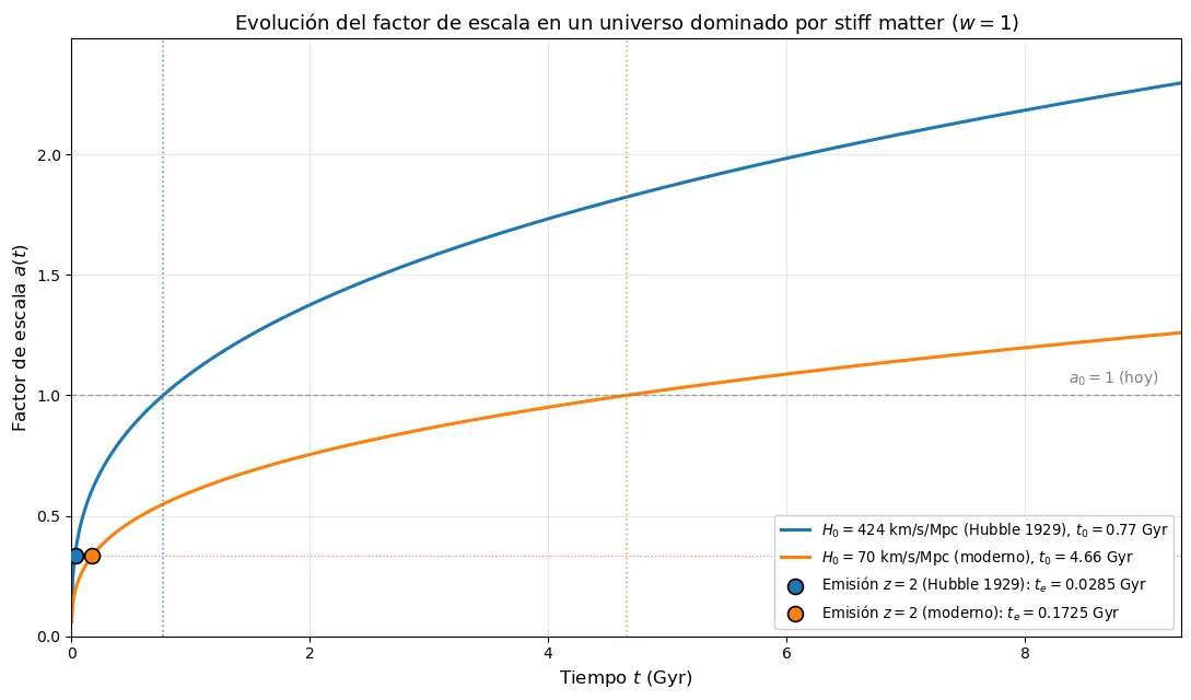
Both curves have the same shape; what changes is how much they are stretched or compressed in real time. With a large H₀, the universe “ages” very quickly: the same phases of expansion take place on shorter time scales. That is why, when they are overlaid in real time, one curve seems to be “ahead” of the other.

Comparison between the two values of H₀

All the cosmological observables calculated in this model depend inversely on the Hubble constant. The closed expressions obtained are summarised as:

t₀ = 1/(3H₀), d_h = c/(2H₀), d_p(z = 2) = 4c/(9H₀), t_e(z = 2) = t₀/27

That is, doubling H₀ halves the age, the size of the observable universe and the distance to a given source. Since the value obtained from Hubble’s data (1929) is about 6 times larger than the modern reference value (424 versus 70 km/s/Mpc), the resulting universe in that scenario is proportionally younger (0.77 Gyr versus 4.66 Gyr) and smaller (354 Mpc versus 2141 Mpc for the particle horizon).

This difference directly illustrates the quantitative impact of the historical overestimate of H₀ discussed in the first section: a disproportionately high Hubble constant not only shifts the numerical values but would produce a stiff-matter universe so young (~770 million years) that it would be incompatible with the observed age of the oldest known stars in the Milky Way itself (~13 Gyr; Bond et al., 2013).

Conclusions on the w = 1 model

The quantitative analysis allows several conclusions to be drawn about the properties of a universe dominated by stiff matter:

• The energy density decays as ρ ∝ a⁻⁶, faster than radiation (a⁻⁴) or non-relativistic matter (a⁻³). A stiff-matter component loses cosmological relevance with expansion at a rate unmatched among physical fluids: if it ever dominated, its relative contribution falls extremely fast as the universe stretches.
• The scale factor grows as a ∝ t^1/3, more slowly than with matter (t^2/3) or radiation (t^1/2). The expansion is vigorous at first but soon flattens, a reflection of the strong self-gravity of a fluid with such high pressure.
• The deceleration parameter q = 2 reaches the maximum value allowed by general relativity for a perfect fluid, corresponding to the causal limit w = 1, at which the speed of sound equals the speed of light. Any larger value of q would require w > 1 and would violate causality. The expansion is therefore decelerated in the most extreme way possible among physically admissible models.
• The age of the universe obtained with H₀ = 70 km/s/Mpc is ≈ 4.66 Gyr, less than a third of the real measured age, ~13.8 Gyr (Planck Collaboration et al., 2020), which confirms that the real universe is not dominated by stiff matter.
• Despite its irrelevance in present-day cosmology, this type of fluid may have dominated at very early epochs, even before the radiation era (Zel’dovich, 1962), when energy densities were high enough for the associated pressure to compete with the energy density itself. Studying it is therefore not a purely academic exercise: it provides intuition about regimes of the early universe that are hard to explore directly and offers an extreme reference against which to contrast other cosmological models.

3. Redshift and temperature of recombination and decoupling

This section leaves the stiff-matter model behind and considers a realistic physical scenario: the early universe dominated by radiation and baryonic matter coupled through Thomson scattering. The aim is to determine, first, the recombination redshift, the moment when free protons and electrons combine to form neutral hydrogen; and, second, the decoupling redshift, when the mean free path of photons becomes larger than the Hubble horizon and the cosmic background radiation is free to propagate to us (Dodelson, 2003; Mukhanov, 2005). The formulation of Unit 6 of the course (Gil-Merino y Rubio, 2024) is followed, applying the Saha equation in its classroom form and the decoupling condition Γ = H.

In thermodynamic equilibrium, the ionisation fraction of hydrogen is obtained from the Saha equation (Saha, 1920), which balances the ionisation and recombination rates. The physical constants are loaded in the corresponding system (energies in eV, cross-sections in m², distances in m), together with the cosmological parameters:

• Present CMB temperature: T₀ = 2.7255 K, measured by COBE/FIRAS (Fixsen, 2009).
• Baryon-to-photon ratio: η = 10⁻⁹.
• Matter density parameter: Ω_m,0 = 0.3, consistent with the ΛCDM model (Planck Collaboration et al., 2020).

The two values of H₀ already used are considered: H₀ = 424 km/s/Mpc, fitted from Hubble’s data (1929), and H₀ = 70 km/s/Mpc as the modern reference value.

The ionisation fraction is defined as:

X ≡ n_e / (n_p + n_H) = n_e / n_B

where X = 1 corresponds to a fully ionised plasma and X = 0 to fully neutral hydrogen. The Saha equation, in the form of equation (5) of Unit 6 (Gil-Merino y Rubio, 2024), relates X to the temperature T and to η:

(1 − X) / X² = 3.84 · η · (kT / m_ec²)^3/2 · exp(Q / kT)

where Q = 13.6 eV is the ionisation energy of hydrogen and m_ec² = 511 keV the rest energy of the electron. Once T is obtained, the redshift is calculated from T(z) = T₀(1 + z), a relation that follows from the conservation of the entropy of the photon fluid during adiabatic expansion (Weinberg, 2008):

z = T / T₀ − 1

It is important to note that the Saha equation is a condition of local thermodynamic equilibrium and does not contain H₀. The recombination redshifts obtained are therefore identical for both values of H₀, as confirmed below.

X	Trec (K)	zrec
0.9	4092.3	1501
0.5	3806.7	1396
0.1	3476.1	1275

Table 4. Recombination (η = 10⁻⁹, independent of H₀).

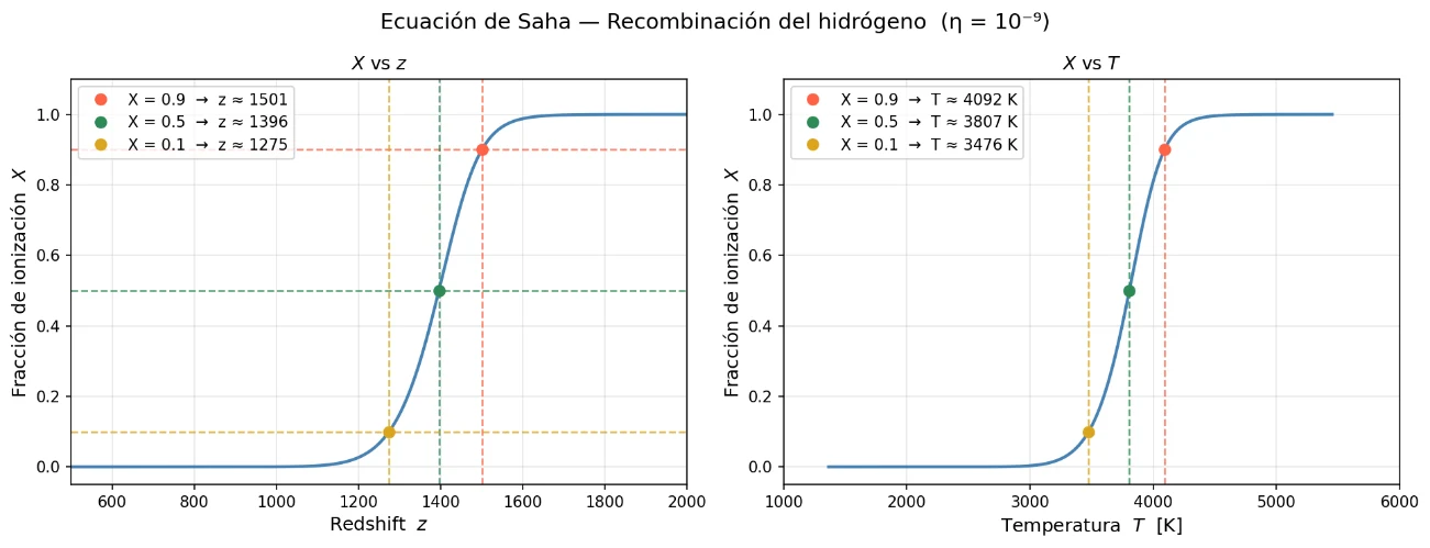
The ionisation fraction goes from 90 % to 10 % over a narrow interval, Δz ≈ 230, which justifies the intuitive idea of recombination as a “fast” process on a cosmological scale. The conventional value X = 0.5 places recombination at z ≈ 1396, in good agreement with the standard literature (Peebles, 1968; Mukhanov, 2005).

Thomson scattering rate. The photons of the radiation bath interact with the free electrons through Thomson scattering (Rybicki and Lightman, 1979). The interaction rate per photon is:

Γ(z) = n_e(z) σ_T c = X(z) n_B(z) σ_T c

with σ_T = 6.65 × 10⁻²⁹ m² the Thomson cross-section. Using the fact that the baryon density scales as n_B(z) = n_B,0(1 + z)³ and substituting n_B,0 = Ω_B,0 ρ_c,0 / m_p with Ω_B,0 = 0.04, the closed expression of Unit 6 is obtained (Gil-Merino y Rubio, 2024):

Γ(z) = 4.4 × 10⁻²¹ · X(z) · (1 + z)³ [s⁻¹]

Hubble parameter in matter domination. In the range z < z_eq relevant to recombination, the universe is dominated by non-relativistic matter and the Friedmann equation reduces to (Liddle, 2015):

H(z) = H₀ √Ω_m,0 · (1 + z)^3/2

Here H₀ does enter explicitly, and this is where the dependence of decoupling on the adopted value of the Hubble constant comes from.

Decoupling between matter and radiation occurs when the scattering rate of a photon equals the expansion rate of the universe (Dodelson, 2003): Γ(z_dec) = H(z_dec). Substituting the previous expressions and imposing the equality gives the implicit equation:

1 + z_dec = [H₀ √Ω_m,0 / (4.4 × 10⁻²¹ · X(z_dec))]^2/3

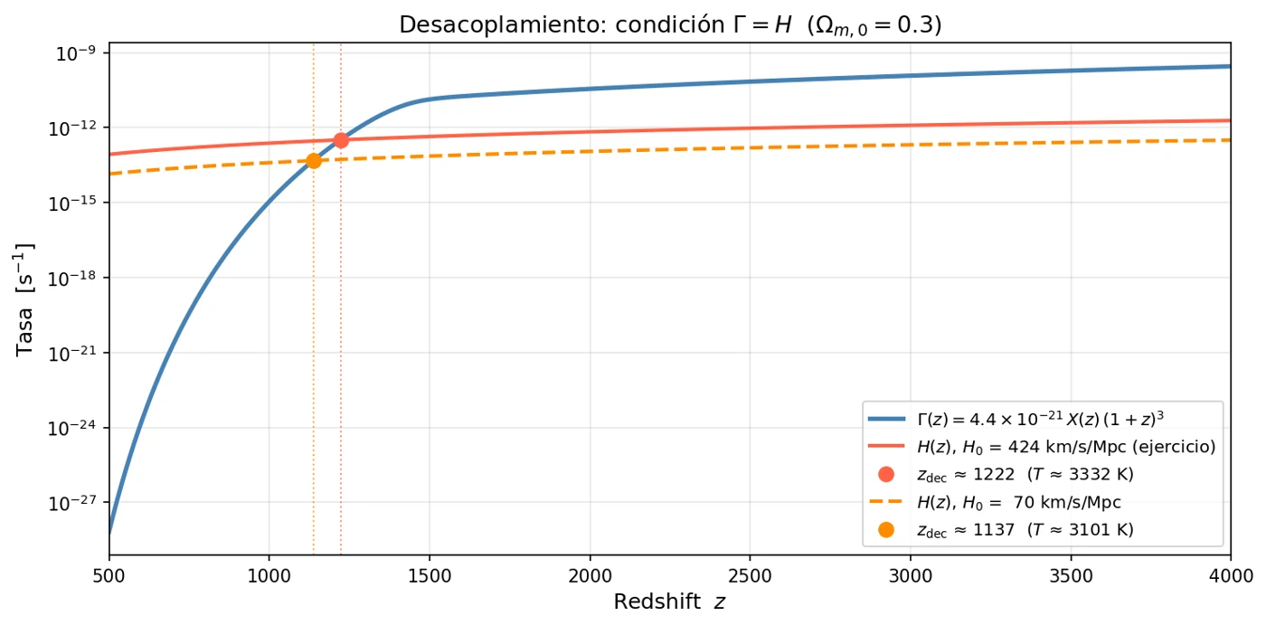
It is solved numerically, because X(z) also depends on z through the Saha equation. The associated temperature is T_dec = T₀(1 + z_dec). A larger H₀ implies faster expansion, so Γ = H is reached earlier (at higher z), which gives earlier decoupling.

H₀	zdec	Tdec (K)
424 km/s/Mpc (exercise)	1222	3332.2
70 km/s/Mpc	1137	3101.2

Table 5. Decoupling (Ω_m,0 = 0.3).

Ionisation fraction X(z) according to the Saha equation. The solution of the Saha equation is plotted below over the range z ∈ [500, 2000], marking the three milestones of the recombination process (X = 0.9, 0.5 and 0.1), both as a function of redshift and of temperature.

Decoupling condition: Γ(z) against H(z). By overlaying on a logarithmic scale the Thomson scattering rate Γ(z) and the Hubble parameter H(z) for both values of H₀, the intersection that defines z_dec can be identified graphically. For H₀ = 424 km/s/Mpc the H curve is shifted upwards overall (the expansion is about six times faster at every z), so the equality Γ = H is reached at a considerably higher redshift.

Bringing together the results of the two calculations: recombination is independent of H₀ (it depends only on η and on atomic constants), whereas decoupling does depend on the adopted value of the Hubble constant.

Quantity	Condition	H₀ = 424 km/s/Mpc	H₀ = 70 km/s/Mpc
zrec (X = 0.9)	Start of recombination	1501	1501
zrec (X = 0.5)	Midpoint	1396	1396
zrec (X = 0.1)	End of recombination	1275	1275
zdec	Γ = H	1222	1137
Tdec	T₀(1 + zdec)	3332 K	3101 K

Table 6. Recombination (Saha equation) and decoupling (condition Γ = H), calculated with η = 10⁻⁹ and Ω_m,0 = 0.3.

For comparison, the simplified model of Unit 6 of the course (Gil-Merino y Rubio, 2024), with η = 5.5 × 10⁻¹⁰ and H₀ = 67.4 km/s/Mpc, obtains:

• z_rec ≈ 1375 (with X = 0.5).
• z_dec ≈ 1140.

This is in reasonable agreement with Planck’s canonical value for the last-scattering surface, z* ≈ 1090 (Planck Collaboration et al., 2020).

Conclusions on recombination and decoupling

Recombination does not depend on H₀. The Saha equation is a condition of local thermodynamic equilibrium that involves only T, η and atomic constants. This explains why the recombination redshifts in Table 6 are identical for both values of H₀: the microscopic physics of the hydrogen atom does not “know” how fast the universe is expanding (Mukhanov, 2005).

Decoupling does depend on H₀, although weakly. The condition Γ = H involves the Hubble parameter. If the ionisation fraction X were constant, the implicit equation would give the scaling 1 + z_dec ∝ H₀^2/3, and a factor of six in H₀ would translate into a factor of 6^2/3 ≈ 3.3 in (1 + z_dec). But X(z) plummets during recombination and absorbs almost all of the effect: the real dependence is much weaker (1223/1138 ≈ 1.07). As Table 6 shows, with H₀ = 424 km/s/Mpc decoupling occurs at z ≈ 1222 (T ≈ 3332 K), noticeably earlier than with H₀ = 70 km/s/Mpc (z ≈ 1137, T ≈ 3101 K).

Time order: why z_dec ≲ z_rec. The density of free electrons n_e = X n_B does not drop to zero instantly when recombination ends: a small residual fraction of ionised hydrogen remains and keeps scattering photons. Decoupling happens somewhat later, when that residual fraction is low enough for Γ < H. In the canonical ΛCDM model this translates into z_rec ≈ 1100 and z_dec ≈ 1085 (Hu and Dodelson, 2002; Planck Collaboration et al., 2020). The simplified model reproduces this order qualitatively, although with somewhat higher numerical values because of the Saha approximation in strict equilibrium (Peebles, 1968).

Final conclusions

The three problems addressed share a common thread: the central role of the Hubble constant H₀ as the parameter that sets the time and space scales of the universe.

In the first, reproducing Hubble’s fit (1929) to the 24 original nebulae gives H₀ ≈ 424 km/s/Mpc (forced through the origin), a value overestimated by a factor of ~6 relative to modern measurements (Planck Collaboration et al., 2020; Riess et al., 2022) for reasons that are now well identified. The difference between the current values from the CMB and from the local scale, the Hubble tension, remains an open problem that could point to physics beyond the ΛCDM model (Verde et al., 2019; Di Valentino et al., 2021).

The second problem showed, through the closed expressions a(t) = (3H₀t)^1/3, t₀ = 1/(3H₀), d_h = c/(2H₀) and q = 2 for a universe dominated by stiff matter (w = 1), that all the observables scale inversely with H₀. The result is a disproportionately young universe in both scenarios (0.77 and 4.66 Gyr), incompatible with the real age of ~13.8 Gyr (Planck Collaboration et al., 2020). The model nevertheless retains teaching value, because it illustrates the causal limit of general relativity and provides intuition about very early epochs (Zel’dovich, 1962).

Finally, the third problem completes the picture by applying the Saha equation together with the decoupling condition Γ = H: a recombination redshift z_rec ≈ 1396 is obtained (independent of H₀, since it is local thermodynamic equilibrium) and a decoupling redshift z_dec ≈ 1222 or 1137 depending on the value of H₀ adopted, in reasonable agreement with z* ≈ 1090 (Planck Collaboration et al., 2020).

This asymmetry, thermodynamic invariance versus kinematic dependence, reveals the separation between the microscopic physics of the hydrogen atom and the global dynamics of the expansion, and it sums up the twofold lesson of the work: H₀ holds the whole cosmological edifice together, but simplified models, although correct to first order, fall short of the current precision of the field, which can discern 5σ tensions between independent methods and perhaps opens the door to new physics waiting to be discovered.

References

• Baade, W. (1952). A revision of the extra-galactic distance scale. Transactions of the International Astronomical Union, 8, 397–398.
• Bond, H. E., Nelan, E. P., VandenBerg, D. A., Schaefer, G. H., & Harmer, D. (2013). HD 140283: A star in the solar neighborhood that formed shortly after the Big Bang. The Astrophysical Journal Letters, 765(1), L12.
• Carroll, S. M. (2004). Spacetime and Geometry: An Introduction to General Relativity. Addison-Wesley.
• Di Valentino, E., Mena, O., Pan, S., Visinelli, L., Yang, W., Melchiorri, A., Mota, D. F., Riess, A. G., & Silk, J. (2021). In the realm of the Hubble tension—a review of solutions. Classical and Quantum Gravity, 38(15), 153001.
• Dodelson, S. (2003). Modern Cosmology. Academic Press.
• Fixsen, D. J. (2009). The temperature of the cosmic microwave background. The Astrophysical Journal, 707(2), 916–920.
• Freedman, W. L., Madore, B. F., Hoyt, T. J., et al. (2025). Status report on the Chicago–Carnegie Hubble Program (CCHP): Measurement of the Hubble constant using the Hubble and James Webb space telescopes. The Astrophysical Journal, 985(2), 203.
• Friedmann, A. (1922). Über die Krümmung des Raumes. Zeitschrift für Physik, 10(1), 377–386.
• Gaia Collaboration, Vallenari, A., et al. (2023). Gaia Data Release 3: Summary of the content and survey properties. Astronomy & Astrophysics, 674, A1.
• Gil-Merino y Rubio, R. (2024). Cosmología y estructura del universo a gran escala. Tema 6: Radiación cósmica de fondo. UNIR.
• Hu, W., & Dodelson, S. (2002). Cosmic microwave background anisotropies. Annual Review of Astronomy and Astrophysics, 40, 171–216.
• Hubble, E. (1929). A relation between distance and radial velocity among extra-galactic nebulae. Proceedings of the National Academy of Sciences, 15(3), 168–173.
• Kolb, E. W., & Turner, M. S. (1990). The Early Universe. Addison-Wesley.
• Liddle, A. (2015). An Introduction to Modern Cosmology (3rd ed.). Wiley.
• Mukhanov, V. (2005). Physical Foundations of Cosmology. Cambridge University Press.
• Peebles, P. J. E. (1968). Recombination of the primeval plasma. The Astrophysical Journal, 153, 1–11.
• Perryman, M. A. C., et al. (1997). The Hipparcos catalogue. Astronomy & Astrophysics, 323, L49–L52.
• Planck Collaboration, Aghanim, N., et al. (2020). Planck 2018 results. VI. Cosmological parameters. Astronomy & Astrophysics, 641, A6.
• Riess, A. G., et al. (2022). A comprehensive measurement of the local value of the Hubble constant with 1 km s⁻¹ Mpc⁻¹ uncertainty from the Hubble Space Telescope and the SH0ES team. The Astrophysical Journal Letters, 934(1), L7.
• Riess, A. G., et al. (2024). JWST observations reject unrecognized crowding of Cepheid photometry as an explanation for the Hubble tension at 8σ confidence. The Astrophysical Journal Letters, 962(1), L17.
• Rybicki, G. B., & Lightman, A. P. (1979). Radiative Processes in Astrophysics. Wiley.
• Ryden, B. (2017). Introduction to Cosmology (2nd ed.). Cambridge University Press.
• Saha, M. N. (1920). Ionization in the solar chromosphere. The London, Edinburgh, and Dublin Philosophical Magazine and Journal of Science, 40(238), 472–488.
• Sandage, A. (1958). Current problems in the extragalactic distance scale. The Astrophysical Journal, 127, 513–526.
• Shapley, H. (1918). Studies based on the colors and magnitudes in stellar clusters. VI. On the determination of the distances of globular clusters. The Astrophysical Journal, 48, 154–181.
• Strauss, M. A., & Willick, J. A. (1995). The density and peculiar velocity fields of nearby galaxies. Physics Reports, 261(5–6), 271–431.
• Trumpler, R. J. (1930). Absorption of light in the galactic system. Publications of the Astronomical Society of the Pacific, 42(248), 214–227.
• Verde, L., Treu, T., & Riess, A. G. (2019). Tensions between the early and the late Universe. Nature Astronomy, 3, 891–895.
• Weinberg, S. (2008). Cosmology. Oxford University Press.
• Zel’dovich, Ya. B. (1962). The equation of state at ultrahigh densities and its relativistic limitations. Soviet Physics JETP, 14(5), 1143–1147.