Simulation and deconvolution of astronomical observations

1. Convolution of the object with the PSF

The universe is sharp, but our “eyes”, the telescopes, are not. To learn how to “clean” images of the cosmos, one first has to understand exactly how they get dirty. In this practical, an ideal image of Saturn was taken as the reference (ground truth, GT) and subjected to a realistic degradation process.

No optical instrument is perfect: because of diffraction, every point of light is blurred into a spot called the PSF (Point Spread Function). This effect was replicated through a convolution, a mathematical operation that redistributes the intensity of each pixel to its neighbours and turns the GT into a degraded observational response. The stochastic nature of the capture was then added through two types of noise:

• Additive white Gaussian noise (AWGN): it represents the electronic readout noise and the thermal noise of the sensor.
• Poisson noise: also known as shot noise, it represents the statistics of photon counting, inherent in the nature of light.

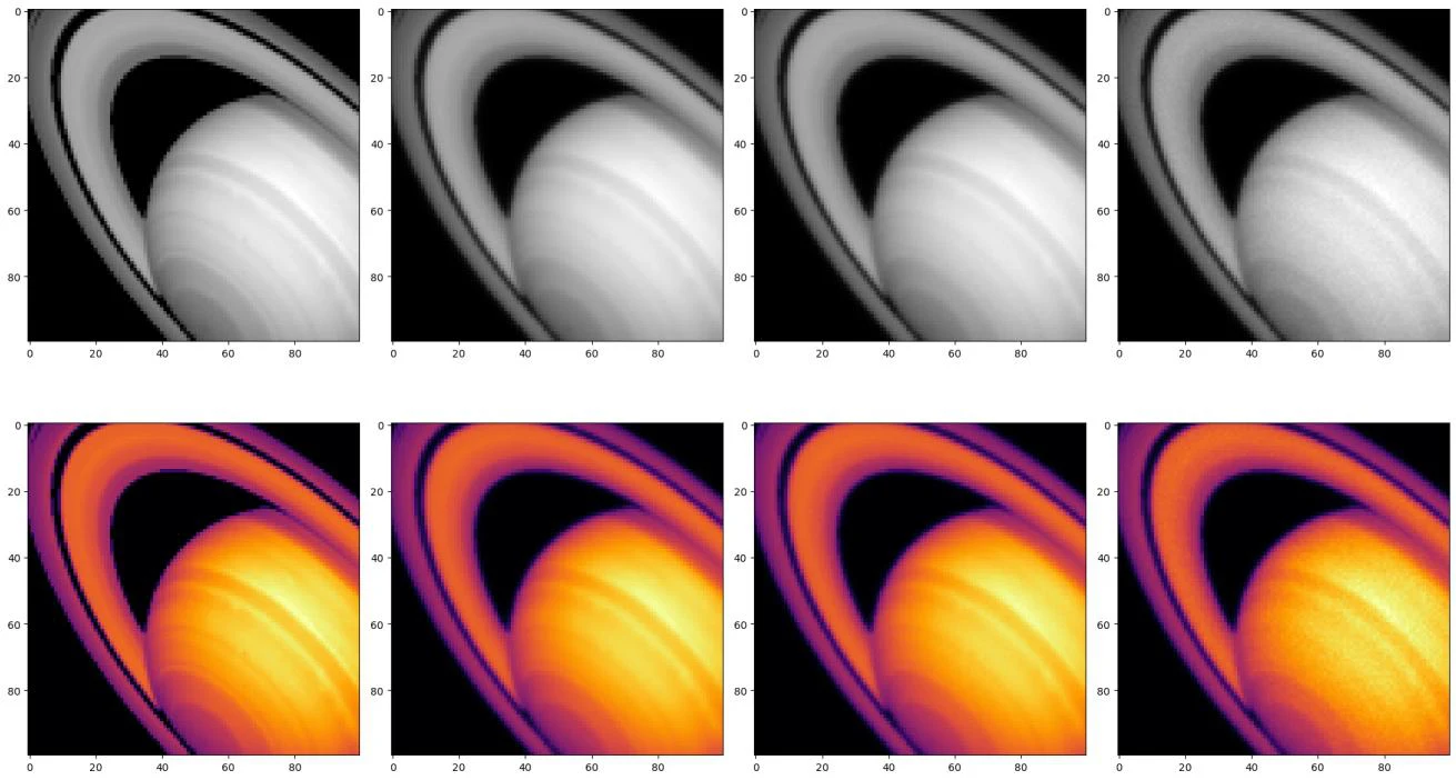
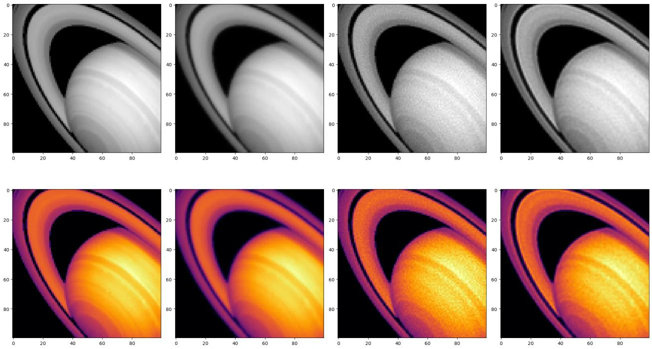
To quantify the degradation, the signal-to-noise ratio (SNR) was calculated in each case (Table 1 of Appendix I). Both simulations share an SNR close to ~7.8; starting from this equivalent level of “dirt” is key to comparing fairly how two different statistical natures affect image quality. While the mean brightness remains stable, the standard deviation reveals the size of the uncertainty introduced: the perfect pixels of the GT have turned into a “real” capture (Image 1 of Appendix II), in which the scientific signal struggles to stand out against the grain and the blur.

2. Supervised Wiener restoration

The next challenge is to reverse the damage. Supervised Wiener restoration is an algorithm that seeks a mathematical balance between two problems: focusing the image (undoing the PSF) without amplifying the noise. It is called “supervised” because the regularisation parameter K must be calibrated manually. To assess the fidelity of the reconstruction against the GT, the mean squared error (MSE) was used: the lower it is, the better the restoration. Applying several values of K revealed an interesting behaviour:

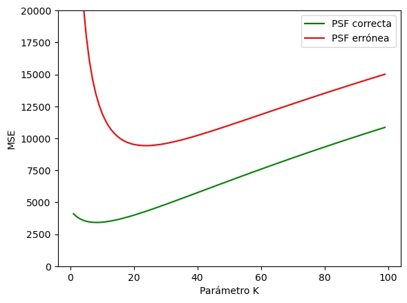
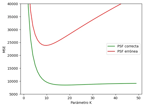
• With the correct PSF: the optimum is reached at K = 8, with a minimum MSE of 3418.44. Physically, this is where the maximum detail of the rings is recovered before the electronic noise destroys the image.
• With the wrong PSF: the algorithm gets lost and its best attempt requires K = 24, stalling at an error of 9428.39, almost three times higher.

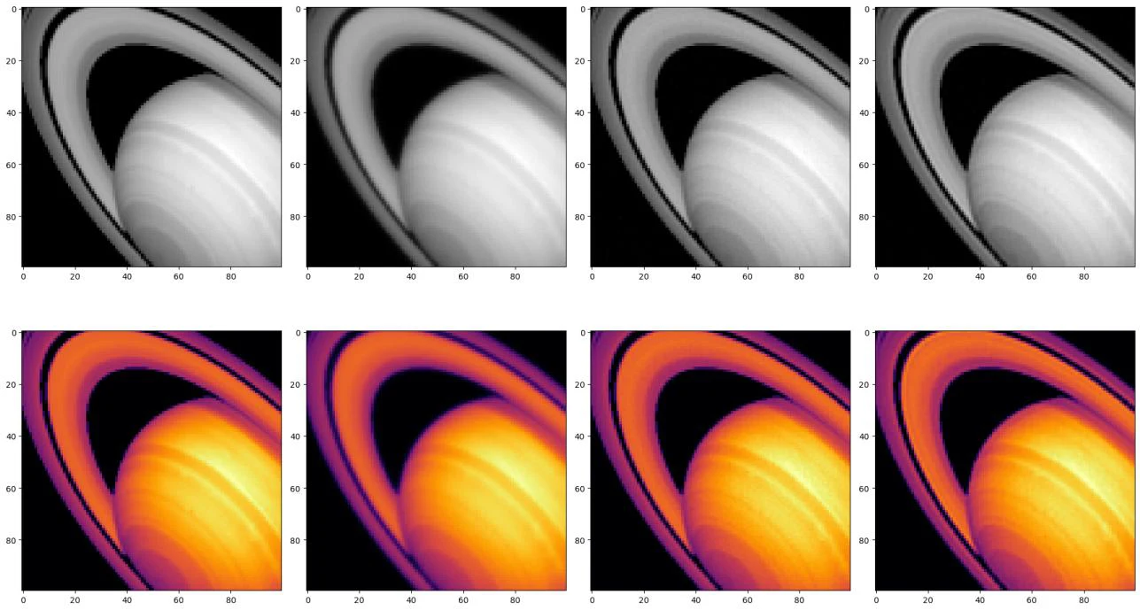
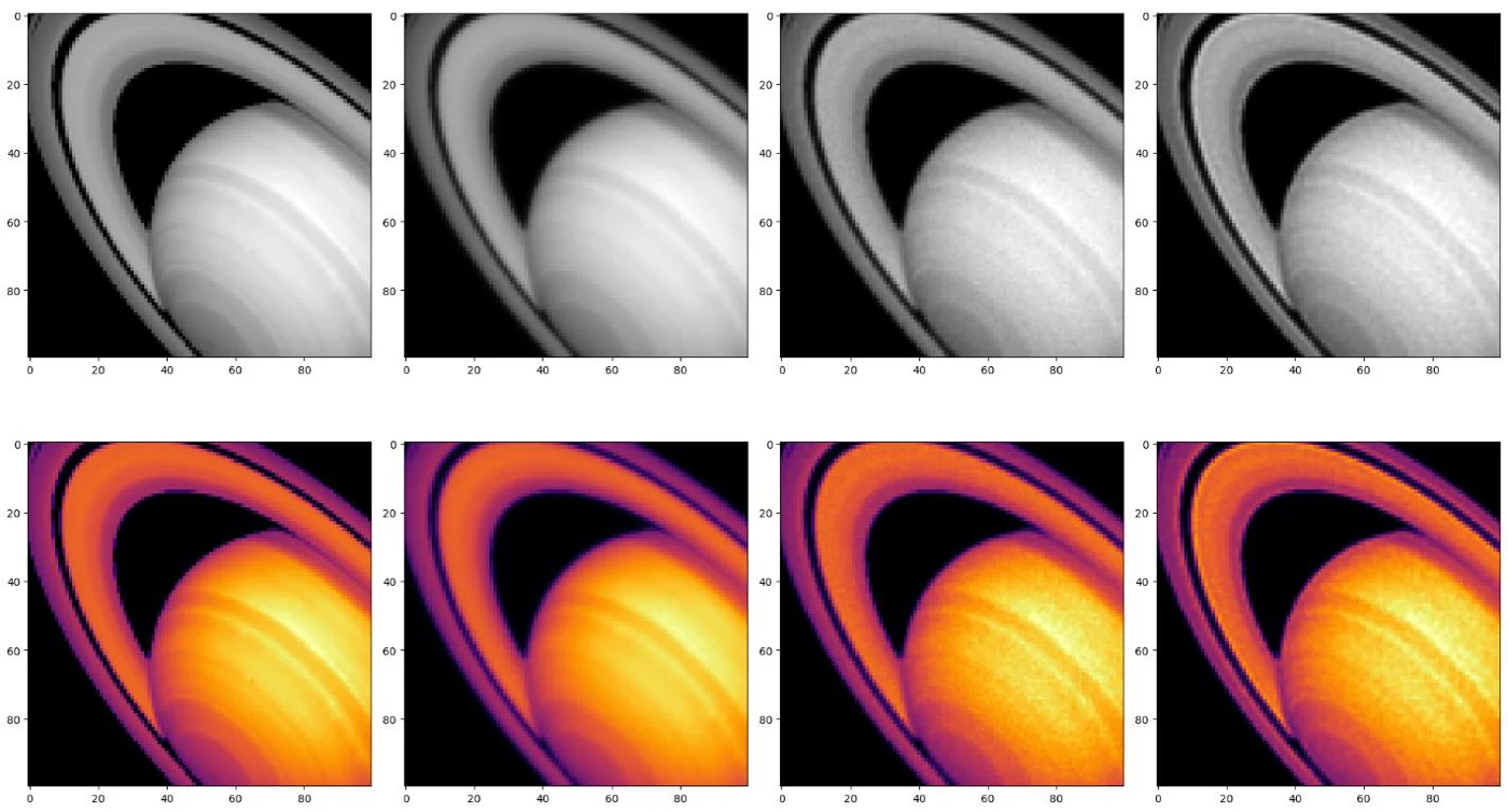
Image 2 of Appendix II shows how, in the red curve, a poor choice of PSF condemns the reconstruction from the start: even at its lowest point, the error remains very high. This shows that knowing the instrument is vital. Image 3 of Appendix II shows the matrix of images after applying the supervised Wiener filter; its interpretation is given in its caption.

Interpretation of the metrics. To validate this recovery quantitatively, two metrics were used: the MSE and the PSNR (peak signal-to-noise ratio), measured in decibels (dB), where a higher value indicates greater fidelity. The results (Table 2 of Appendix I, calculated on the central crop of the image) confirm a clear jump in quality: going from the blurred image to the reconstruction with the correct PSF, the MSE falls drastically (by almost 95 %) and the PSNR rises by almost 13 dB. This means that the Wiener filter has managed to recover a massive amount of structural information “hidden” by the instrumental blur.

3. Unsupervised Wiener restoration

In this case, the algorithm is left to estimate the parameter K automatically, analysing the statistics of the blurred image to separate the real structure of Saturn from the random noise. This is an advantage in real scenarios, where there is no perfect model with which to calculate the MSE.

The results (Image 4 of Appendix II) show a behaviour similar to that of the supervised method, which validates that the algorithm’s automatic estimate is quite accurate, especially with the correct PSF. As before, using the wrong PSF brings back artefacts near the Cassini division and at the edge of the planet. The metrics are given in Table 3 of Appendix I.

Which method gives better results, supervised or unsupervised Wiener? Which would be used in a real situation? Numerically, the supervised method remains superior, with a PSNR of 43.44 dB and an MSE of 4260.49, because it allows one to “cheat” by scanning K against the GT. In real astronomical research, however, the logical choice is unsupervised Wiener: in professional practice the perfect object is not available for tuning parameters by hand. So, although the automatic approach is slightly less accurate, its ability to estimate the signal-to-noise ratio based only on the observed data makes it the most robust and realistic operational tool.

4. Richardson–Lucy restoration

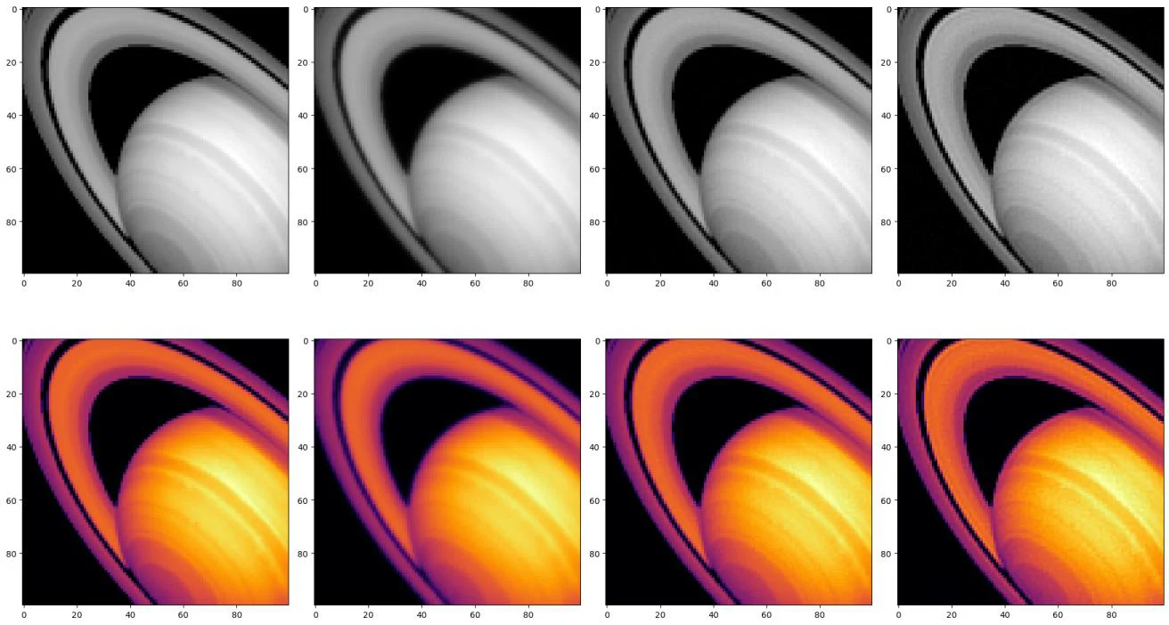
This approach is designed specifically to model Poisson noise. When applied, the algorithm refines the structure of Saturn step by step through successive correction factors. In Richardson–Lucy (RL), the parameter that is tuned is the number of iterations. The analysis of the results reveals a clear semi-convergence behaviour (Image 5 of Appendix II).

Iterations and visual interpretation. K3 = 18 iterations were chosen for the correct PSF and K4 = 10 for the wrong one, for the reasons given. Both reconstructions improve on the blurred image, although less spectacularly than with Wiener. Richardson–Lucy tends to produce more “grainy” results (Image 6 of Appendix II) because it does not explicitly penalise noise. With the correct PSF, the rings stand out from the disc and the brightness gradients of the planet can be seen; with the wrong one, the contrast improves, but the edges appear wavy and small “lumps” appear where there was previously a smooth gradient.

Even so, it was agreed that, visually, the reconstruction with the wrong PSF looks more pleasing than the correct one: not everything that looks “nice” is scientifically correct. Finally, iterating manually with the parameter K3, a value lower than the one giving the minimum produces a better visual result (Image 6b of Appendix II) but worse numerical indicators (Table 4 of Appendix I).

5. Restoration with the wrong statistics

In this test, the algorithms were crossed with noises they were not designed for: the RL algorithm with the AWGN image and the Wiener filter with the Poisson image, always with the correct PSF.

5.1. Wiener with AWGN versus Wiener with Poisson

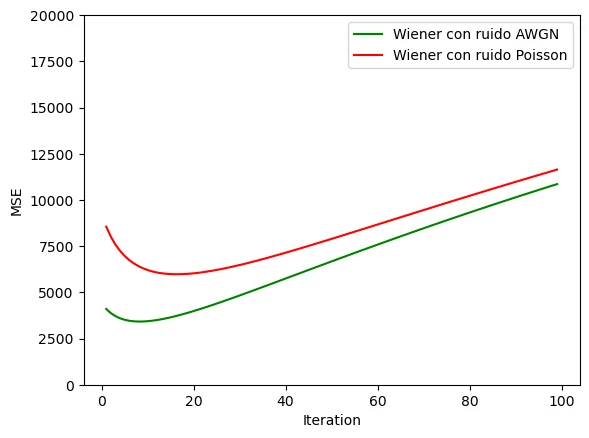
The error curves (Image 7 of Appendix II) show that, although both have the U shape typical of regularisation, the Wiener restoration with Poisson noise always stays above: the filter assumes Gaussian noise and, when it receives Poisson noise, does what it can but carries a model error that no value of K removes. Its PSNR and MSE metrics are given in Table 5 of Appendix I, evaluated at K = 99.

When should the Wiener filter be used with Poisson noise? The evidence shows that it can be used effectively in two specific astronomical scenarios:

• In high-flux regimes: when observing very bright objects, Poisson statistics converge mathematically towards a Gaussian distribution by the central limit theorem, which makes the approximation physically valid.
• In situations with severe computational resource limits: being a linear, single-step method in the Fourier domain, it is orders of magnitude faster than the iterative Richardson–Lucy process, which makes it ideal for processing massive volumes of data (astronomical surveys) or generating real-time previews at the telescope itself.

5.2. RL with Poisson versus RL with AWGN

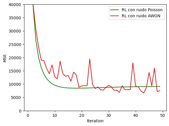
The situation is symmetric to the previous one. Image 8 of Appendix II shows that Richardson–Lucy on Poisson noise, its natural scenario, descends smoothly and stabilises near iteration 18. However, when the algorithm is forced to work with AWGN, the MSE profile suffers strong oscillations and numerical instabilities over the iterations. Since the probabilistic core of Richardson–Lucy is not designed to deal with the homogeneous distribution of electronic noise, the filter interprets the thermal fluctuations of the background as real signals, which causes spurious error peaks and a chaotic behaviour that rules out its use in scenarios of this kind.

6. Realistic restoration of M100

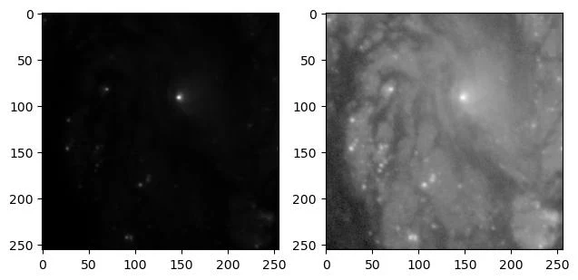
To simulate a realistic observational scenario, the image of the galaxy M100 was imported in FITS format (Image 9 of Appendix II), without knowledge of the instrumental PSF or the GT. The primary statistical analysis revealed a dynamic range of 9 to 7653 counts and an extremely low signal-to-noise ratio (SNR = 1.19).

What noise is it? The grain of the black background is completely homogeneous and fine, and it covers the empty space and the bright areas of the galaxy alike: it is not concentrated only where there is light. It is therefore white Gaussian noise (AWGN).

Since the GT is not available for iterating by hand, the supervised method and blind Richardson–Lucy (which would be chaotic, given the oscillations seen with AWGN) are ruled out, and the appropriate scientific tool is unsupervised Wiener: the filter itself automatically estimates the spatial statistics of the electronic noise. Even so, Richardson–Lucy was also tried for an objective visual comparison.

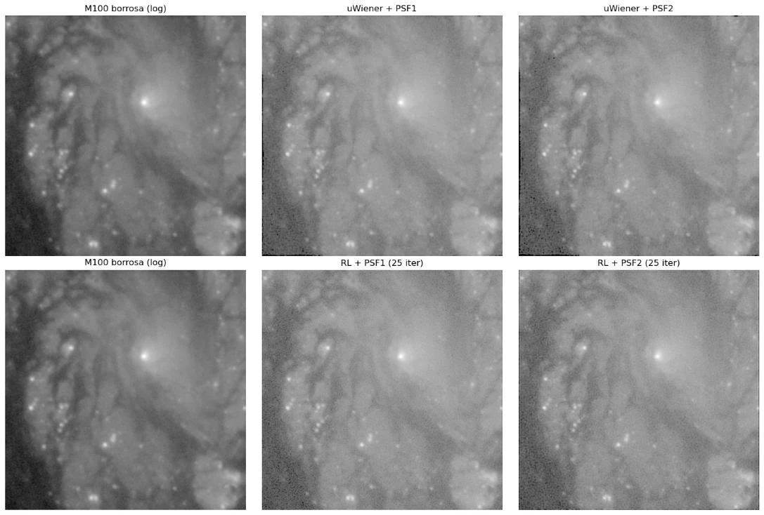
To solve the restoration in a blind scenario, the unsupervised Wiener and Richardson–Lucy algorithms were cross-evaluated against the two candidate PSFs. Visual inspection of the reconstructions (Image 10 of Appendix II) determines that unsupervised Wiener with PSF 1 gives the scientifically optimal restoration. With that combination, the bright points (star clusters) in the spiral arms on the left look smaller, rounder and more compact, that is, better focused; with PSF 2, those same points appear slightly more stretched or blurred and the background looks “dirtier”. PSF 1 is the true optical description of the simulated telescope.

Conclusion

This laboratory shows that the success of astronomical restoration rests on three fundamental pillars, drawn from the Saturn simulations and the real case of M100:

1. Statistical consistency between the algorithm and the physical nature of the noise (AWGN for Wiener and Poisson for Richardson–Lucy) is more critical than the fine-tuning of the parameters itself.
2. Accurate knowledge of the instrumentation (the PSF) is the most decisive factor in the process, since a wrong optical model induces destructive geometric artefacts that cannot be corrected.
3. In real observational scenarios without a reference model (ground truth), unsupervised approaches are the only robust and honest methodological alternative, and they demonstrate their operational viability by estimating the signal-to-noise ratio exclusively from the telescope data.

All the numerical results, plots and restorations were obtained with a Jupyter notebook containing the full code and the reproducible outputs of each step.

Appendix I. Tables

The metrics in these tables were calculated on the central 100 × 100-pixel crop containing Saturn, whereas the MSE curves in Images 2, 5, 7 and 8 were calculated on the whole image. That is why the figures in the tables and those in the curves do not match.

Noise source	SNR	Mean	Standard deviation
Gaussian (AWGN)	7.79	7842.41	1005.91
Poisson (shot noise)	7.76	7843.60	1009.98

Table 1. Quality metrics (SNR) and statistical parameters after adding AWGN and Poisson noise.

Image / reconstruction	PSNR (dB)	MSE
Blurred image (with noise)	30.45	84,769.55
Reconstruction with wrong PSF	36.36	21,743.44
Reconstruction with correct PSF	43.44	4260.49

Table 2. Metrics of the supervised Wiener restoration.

Image / reconstruction	PSNR (dB)	MSE
Blurred image (with noise)	30.45	84,769.55
Reconstruction with wrong PSF	35.49	26,574.09
Reconstruction with correct PSF	42.17	5704.73

Table 3. Metrics of the unsupervised Wiener restoration.

Image / reconstruction	PSNR (dB)	PSNR (dB)*	MSE	MSE*
Blurred image (with noise)	30.45	30.45	84,769.55	84,769.55
Reconstruction with wrong PSF	31.49	31.42	66,703.74	67,804.83
Reconstruction with correct PSF	34.77	33.04	31,359.71	46,754.87

Table 4. Richardson–Lucy metrics with the MSE-optimal iterations (K3 = 18, K4 = 10). *With K3 = 5 (better visual result, worse metric).

Restoration configuration	PSNR (dB)	MSE
Wiener with Poisson noise (wrong statistics)	34.73	31,656.39
Wiener with AWGN noise (correct statistics)	35.52	26,417.91

Table 5. Metrics of the Wiener filter with the correct (AWGN) versus the wrong (Poisson) statistics, with the correct PSF. Both were evaluated at the last value of the regularisation sweep (K = 99), not at the optimum of each case.

Appendix II. Images