Deep learning for the identification of trans-Neptunian objects

Introduction

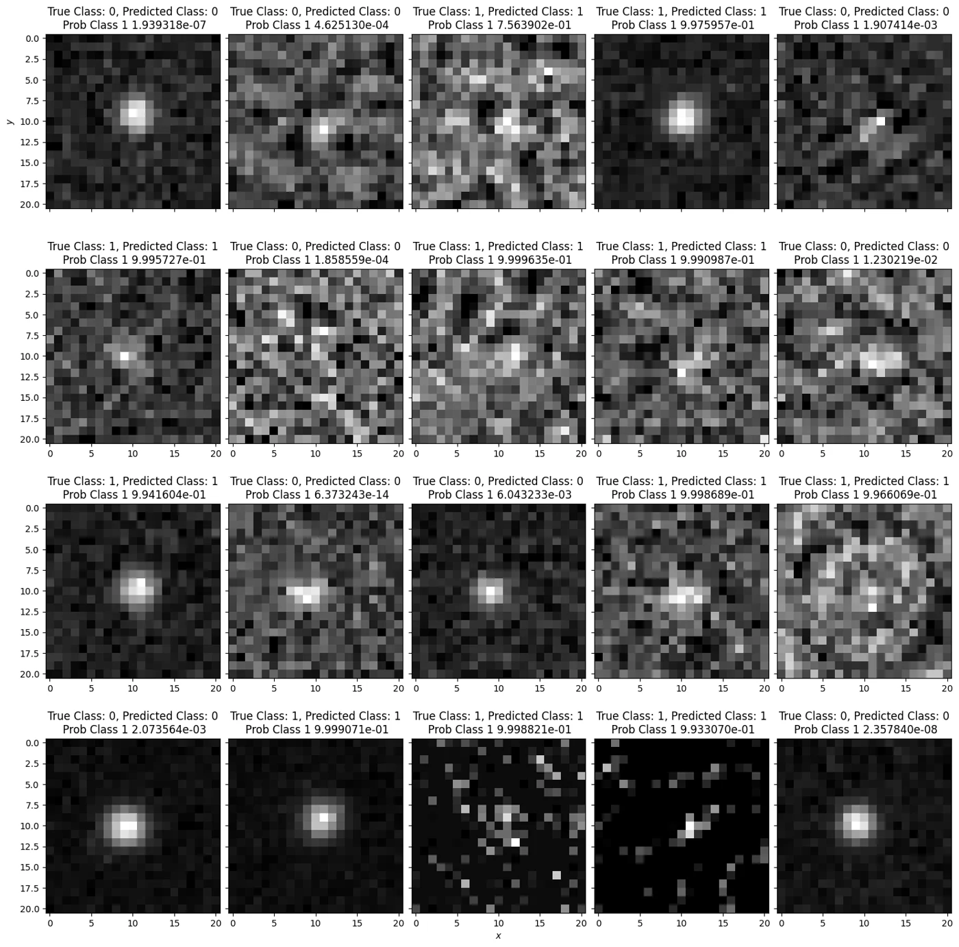
This work tackles a real astronomical problem with deep learning: distinguishing, in small images of 21 × 21 pixels, between true detections of trans-Neptunian objects (TNOs) and false detections produced by noise. The data come from a near-Earth object survey carried out by Lori Allen and collaborators with the DECam camera on the 4 m Blanco telescope (CTIO), and include simulated TNOs (true positives) and tracks with no known sources (false positives), with signal-to-noise ratios from 3 to 100. The aim is to determine how many TNOs there are in the final images. The difficulty is obvious: at low signal-to-noise, a true positive and a false positive are almost indistinguishable by eye, which justifies the use of neural networks.

The set of 109,523 images was split into 80 % for training (87,618), 10 % for validation (10,952) and 10 % for testing (10,953). Of these, 60,000 are simulated TNOs and 49,523 false detections: the TNO class is slightly in the majority (≈ 55 %).

The first part uses a classical fully connected (FC) neural network to study the effect of the optimiser, the batch size and the number of epochs, the interpretation of the confusion matrix and the use of batch normalisation. The second part moves on to convolutional neural networks (CNN): first a VGG6, in which the optimiser hyperparameters are tuned and dropout layers are added, and finally a much deeper architecture, ResNet50, with which an improvement of the result is sought.

I. Part one: fully connected neural network

The starting point is a sequential model with two fully connected hidden layers of 30 neurons and ReLU activation, followed by a 2-node softmax output layer (TNO versus noise). Training consists of finding the weights and biases that minimise the loss function through gradient descent and backpropagation.

1/5. SGD versus ADAM optimiser

Have the TNO images been classified correctly? Why? In this first experiment, the fully connected network is trained with the SGD optimiser and the default values of the exercise: batch size = 1 and a single epoch (epochs = 1), that is, a single pass through the data, updating the weights image by image. Quality is measured with the accuracy (fraction of correctly classified images) and with the loss function, in both training and validation. As a reference, a model is considered well trained when it exceeds ~90 % accuracy.

As Table 1 shows, the model does not classify the TNO images well with the SGD optimiser: the accuracy is around 62 %, far from 90 %. Over different runs, the training accuracy ranged between 62 % and 66 %, with a validation accuracy of about 54–57 %.

Optimiser (batch = 1, 1 epoch)	Training accuracy	Validation accuracy	Training loss	Validation loss
SGD	0.62 – 0.66	0.54 – 0.57	≈ 0.58 – 0.63	≈ 0.68 – 0.70
ADAM	0.93	0.95	0.18 (≈ ⅓ of SGD’s)	0.12

Table 1. Performance of the fully connected network after one epoch with batch size 1, comparing the SGD and ADAM optimisers. For SGD, the range observed over several runs is given; with ADAM, the accuracy exceeds 90 % and the loss falls to about a third.

The main reason for this low accuracy is the combination of the SGD optimiser (sensitive to local minima) with very limited training: with a batch of a single image and a single epoch, the loss function is approximated from a single example per step, so the model does not manage to train properly.

When the experiment is repeated with a second optimiser, does the result improve or get worse? Why that optimiser? For the second experiment, the ADAM optimiser was chosen, as it is the most common first choice and one of the best of the “simple” methods (improved versions exist, such as ADAMW, among others). With it, the result improves enormously: an accuracy above 90 % is reached, with a loss close to a third of that obtained with SGD. In addition, in validation the accuracy increases and the loss decreases, which confirms that the model is well trained.

2/5. Batch size and number of epochs

Does the classification improve compared with n_epochs = 1 and batch_size = 1? Why? How do the numbers evolve during training? Is there overfitting? Exactly the same network and the same SGD optimiser as in the previous section are kept; the only thing that changes is the training regime: the batch size goes from 1 to 435 and the number of epochs from 1 to 200. A batch is the subset of images used to calculate the gradient and update the weights at each iteration; an epoch is a full pass through the whole training set. With 87,618 images and batches of 435, each epoch is about 202 iterations.

This gives a better classification: by increasing the batch size and the number of epochs, the loss function is minimised better. An accuracy of 91.61 % is obtained in training and 91.02 % in validation, with loss values of 0.2444 and 0.2575, respectively.

As for how the numbers evolve: at each iteration the loss is calculated on a batch and the weights are updated, and that result is the starting point for the next batch. Consequently, within each epoch the loss decreases iteration by iteration and the accuracy improves, and each new epoch starts from the result of the previous one. It should be noted that a good result would have been reached with far fewer epochs.

No overfitting is observed: the validation accuracy follows the training accuracy (it is barely half a point lower). It is worth pointing out, however, that in some runs the model starts stuck at ≈ 0.55 (the accuracy obtained by always predicting the majority class) and does not progress; this is attributed to a poor initialisation that falls into a local minimum, and it is solved by restarting the training or redoing the split.

3/5. Confusion matrix and F1-score

How is the confusion matrix interpreted? What is the value of the F1-score?

• Accuracy ≈ 0.92.
• Sensitivity (recall) = TP / (TP + FN) = 0.92 / (0.92 + 0.08) = 0.92.
• Specificity = TN / (TN + FP) = 0.92 / (0.92 + 0.08) = 0.92.
• Precision = TP / (TP + FP) ≈ 0.93, taking into account that 55 % of the images are TNOs: 0.92 · 0.548 / (0.92 · 0.548 + 0.08 · 0.452).

These values indicate a very homogeneous model, with an accuracy of 92 %: it gives no more false positives than false negatives, so it shows no bias in this respect. With a precision of 0.93 and a sensitivity of 0.92, the F1-score is:

F1 = 2 · (precision · sensitivity) / (precision + sensitivity) = 2 · (0.93 · 0.92) / (0.93 + 0.92) ≈ 0.93

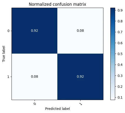
In the matrix, the rows are the true class and the columns the predicted one; class 0 corresponds to false positives (noise) and class 1 to true positives (TNO). The diagonal holds the hits: 92 % of the noise is classified as noise and 92 % of the TNOs as TNO. The errors are symmetric (8 % and 8 %), which is why the model shows no bias towards either class.

4/5. Training curves

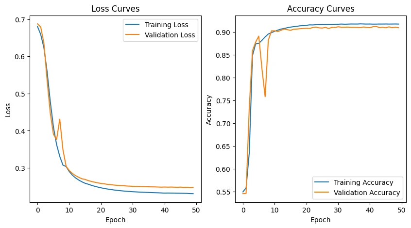
What do the plots show? Is there overfitting? The first plot shows the evolution of the loss function: it drops sharply in the first epochs and then decreases very slowly until it stabilises at ≈ 0.25. The training loss (blue) and the validation loss (orange) are shown; they remain practically superimposed, with validation barely above at the end. The second plot shows the accuracy, with the opposite behaviour: it jumps to ≈ 0.90 in the first epochs and then improves very slowly to ≈ 0.91. Most of the learning happens in the first epochs, which confirms that a similar result would have been reached with considerably fewer epochs.

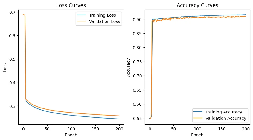
There is no overfitting in this case. The sign of overfitting would be the training curve continuing to improve while the validation curve stalls or gets worse, opening a growing gap between them. Here the opposite happens: the training and validation curves evolve together and in parallel throughout, with a minimal difference (≈ 0.916 versus ≈ 0.910 accuracy). The model generalises equally well to unseen data.

5/5. Batch normalisation

Has batch normalisation improved the classification of the TNO images? Batch normalisation (BN) normalises the activations of the layer so that they have mean 0 and variance 1, which stabilises and speeds up training. To assess its effect, the training of the same network was repeated, with the same SGD and the same batch size of 435, but with BN and only 50 epochs (compared with 200 in the previous section).

The final accuracy barely changes: it stays at ~92 % (0.91 → 0.917), with a precision of 0.93 and a sensitivity of 0.91. That is, BN does not noticeably improve the accuracy, but it does speed up convergence considerably: as the plots show, the minimum of the loss and the maximum accuracy are reached in very few epochs, and the validation curve almost coincides with the training curve. The same ~92 % that previously required 200 epochs is thus achieved in a fraction of the epochs.

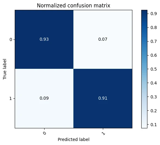
This observation is worth keeping in mind: in this simple, well-integrated network, batch normalisation helps. In the second part it will be seen that the same technique, in a different context, can behave very differently.

II. Part two: convolutional neural networks (CNN)

Convolutional networks are designed to work with images: instead of connecting each neuron to the whole image, they apply filters (kernels) to small regions, which reduces the complexity and provides some invariance to small translations. Their basic components are the convolutional layers, the non-linear activation functions, the pooling layers (which summarise regions, typically with max pooling) and the final fully connected layers. First a VGG6 architecture is used and, finally, a ResNet50.

1/3. VGG6: default parameters and optimiser tuning

Results with the default optimiser parameters. With the default parameters (learning rate = 0.01, momentum = 0.75, nesterov = False), and using the same epoch and batch-size values as in the first part to allow comparison, the VGG6 gave a surprisingly worse result: the accuracy did not exceed 65 % in any of the attempts. It was therefore a poor model for this exercise.

Tuning the learning rate and momentum. From there, several steps were followed:

• The learning rate was reduced to 1e-6, with a somewhat better result, but without reaching 70 %.
• The number of epochs (50) and the batch size (64) were also changed and different momentum values were tried, without improving the result. From this point on, the results shown in Table 2 began to be recorded.
• Even 500 and 1000 epochs were tried, without success.
• Finally, the batch size was set back to 256, with 50–100 epochs, raising the learning rate again to 0.01 (because the smaller it was, the less the learning progressed and the more epochs it needed) and lowering the momentum from 0.75 to 0.5, since, by smoothing the gradient slightly, this parameter favoured learning.

Even so, these changes alone did not give a good result. At that point it was noticed that the outputs themselves were giving clues. A careful review of the metrics revealed a recurring pattern: although the training accuracy could rise, the validation behaved erratically and inconsistently with it. The val_loss shot up to huge values (of the order of thousands) and the val_accuracy oscillated around chance level (Figure 4), while the confusion matrix showed that the model assigned a single class to all the examples. In other words, the model seemed to learn on the training data but was unable to generalise.

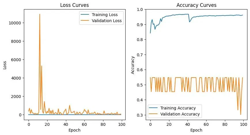
That marked discrepancy between training and validation was the key clue, and it led to suspicion of the BatchNormalization layer. During training this layer normalises the activations with the mean and standard deviation of the batch, but in validation it uses a moving average of those statistics accumulated during training. With a single isolated BatchNormalization layer and an initially unstable training, that moving average was poorly estimated: the network normalised with a different “rule” when validating and its outputs went out of control. This explained why it trained well but failed completely in validation.

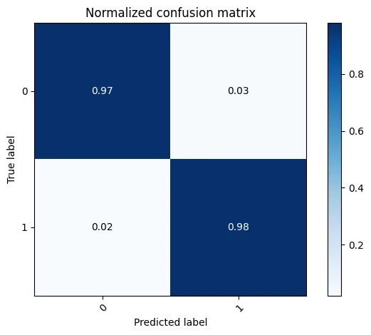
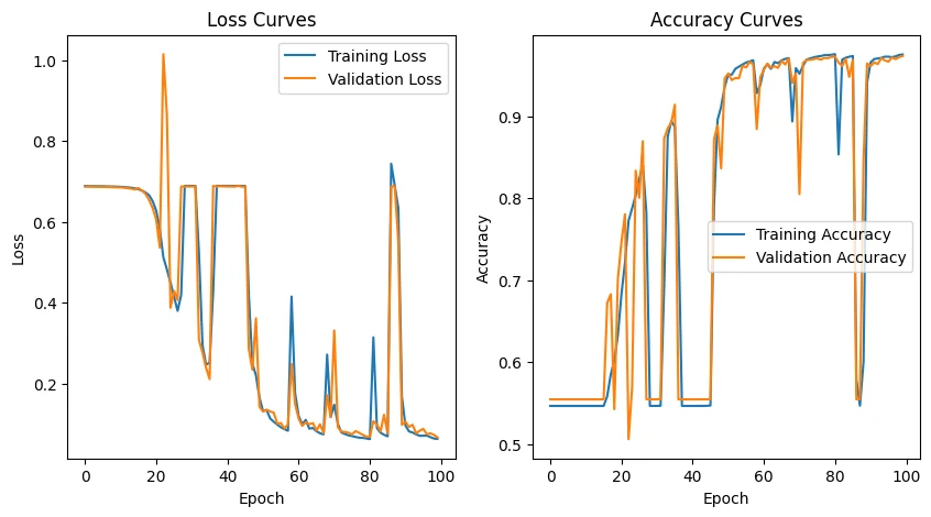
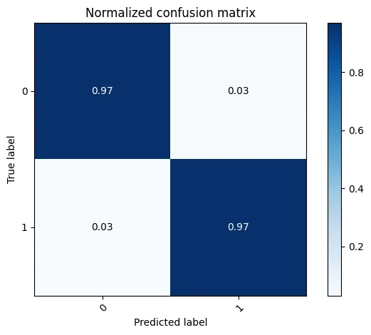
When the BatchNormalization line was commented out, the network performed the same calculation in training and validation, and the instability disappeared. With the final configuration (learning rate = 0.01, momentum = 0.5, nesterov = True, batch size = 256 and 100 epochs, without BatchNormalization), the model converged correctly: the training and validation curves rise together to ≈ 0.97 accuracy (a sign that there is no overfitting) and the loss falls to ≈ 0.07. The final confusion matrix reaches 0.97 and 0.98 hits per class. Although occasional spikes can be seen in the curves (noise typical of SGD), the model recovers from them and keeps converging (Figure 5).

The predictions on individual images (Figure A1 in the Appendix) confirm the good performance: both compact, centred sources and more diffuse, noisy fields are classified correctly.

In conclusion, the good result does not come from a single parameter but from the combination: a learning rate large enough (0.01) to learn without needing an excessive number of epochs; a moderate momentum (0.5) that smooths progress without the optimiser “overshooting”; a large batch size (256) that stabilises the curves; and enough epochs (100) to converge. But the decisive factor was identifying that the BatchNormalization layer was sabotaging generalisation: once it was removed, all the other adjustments could finally show up in a stable, reproducible model with an accuracy close to 97 %. Unlike the simple network of the previous section (where BatchNormalization, well integrated and with stable training, sped up convergence), here it is a single isolated layer with an initially unstable training, conditions under which its moving statistics are poorly estimated and the layer goes from helping to harming.

2/3. Dropout layers

Does the previous classification improve with dropout layers? In terms of accuracy, no. The model with dropout reaches practically the same result as without it: ≈ 97 % in both cases (confusion matrix 0.97/0.97 with dropout versus 0.97/0.98 without). The difference is within the noise of the training itself.

Dropout is a regularisation technique whose function is to reduce overfitting, that is, to close the gap between the (high) training accuracy and the (lower) validation accuracy. The dropout layer randomly zeroes a fraction of the neurons (25–50 %) at each training step, which forces the network not to depend on specific neurons. In this model that gap practically did not exist: even without dropout, the training and validation curves evolved together (once the BatchNormalization layer had been removed). Since the model was not overfitting, dropout had no room to improve the accuracy: a generalisation that is already good cannot be improved.

What dropout did provide was robustness and reproducibility: without it, the results were more variable between runs (in some, training became unstable and collapsed to the trivial solution, ~0.77 and then the majority class), whereas with dropout the good result was obtained consistently and reproducibly (Figure 6).

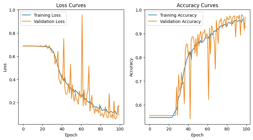
In conclusion, dropout did not improve the accuracy (the model already generalised well without it), but it made the good result more stable and reproducible; it does no harm and it is good practice to keep it. Table 2 summarises the path followed in tuning the VGG6, during which two opposite problems appeared: with too small a learning rate, the model barely moved (the loss did not drop below 0.69), whereas with a high learning rate but a high momentum it learned for a few epochs and then quickly “overshot”, collapsing again to the majority class. The balance appeared with learning rate = 0.01 and momentum = 0.5.

Test	Learning rate	Momentum	Nesterov	Batch	Epochs	Dropout	Result
Default	0.01	0.75	False	64	50	No	Does not learn: stuck always predicting the majority class (acc ≈ 0.547; loss ≈ 0.69).
1	0.00001	0.75	True	64	50	No	Too slow: the loss barely falls and does not get below 0.69.
2	0.001	0.9	True	64	50	No	Learns for a few epochs (val acc ≈ 0.85) and collapses again to the majority class.
3	0.0001	0.5	True	64	50	No	Too slow; hardly progresses.
4	0.01	0.5	True	64	50	Yes	Learns (acc ≈ 0.68), but with very noisy curves that are still rising.
5	0.01	0.5	True	256	100	Yes	Converges stably and reproducibly: training/validation acc ≈ 0.95–0.97; matrix 0.97/0.97.
6	0.01	0.5	True	256	100	No	Variable: in some runs it converges to ≈ 0.97 (matrix 0.97/0.98); in others it becomes unstable and collapses (~0.77 → 0.547). Figure 5.

Table 2. Summary of the VGG6 tuning process: combinations of learning rate, momentum, nesterov, batch size, epochs and dropout evaluated, with the result obtained in each case.

Tests 5 and 6 are the clean comparison of dropout: the same configuration in everything, with the only difference being whether it is enabled. Test 5 was reproduced several times and always gave ≈ 0.97; test 6 gave different results depending on the random initialisation, which shows the stabilising effect of dropout. All the tuning tests used nesterov = True; the “Default” row uses the initial optimiser parameters (learning rate = 0.01, momentum = 0.75, nesterov = False) with the batch size and epochs with which the tests began to be recorded (64 and 50). The BatchNormalization layer, present in the original model, was removed after the first tests because it destabilised the validation; tests 1–6 are already without it.

3/3. ResNet50 versus VGG6

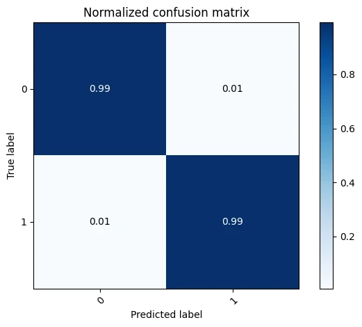
Does the ResNet improve on the TNO classification made by the VGG? Yes, the ResNet50 clearly improved the classification.

Metric	VGG6 (best configuration)	ResNet50
Validation accuracy	≈ 0.97	≈ 0.99
Confusion matrix	0.97 / 0.97	0.99 / 0.99
Epochs to converge	≈ 100 (after much tuning)	≈ 99 % already at epoch 3
Optimiser	Tuned SGD (lr 0.01; momentum 0.5; nesterov)	Default SGD (untuned)
Computational cost	Low (6 layers, ~2 s per epoch)	High (50 layers, ~19 s per epoch)

Table 3. Comparison of the performance of the VGG6 (in its best configuration) and the ResNet50 in the classification of TNOs.

• Improvement in accuracy: from ≈ 97 % (VGG6) to ≈ 99 % (ResNet50). In terms of error, it drops from ≈ 3 % to ≈ 1 % per class, that is, it is reduced to about a third. In TNO detection, where both false positives and missed real detections should be minimised, that reduction is significant.
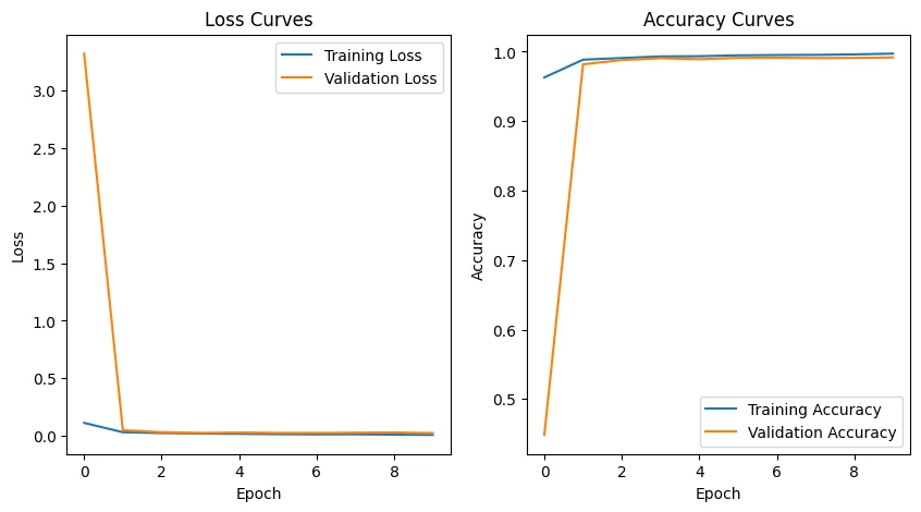
• Much faster learning: the ResNet reached ≈ 99 % already at epoch 3, whereas the VGG needed ≈ 100 epochs and fine tuning of the learning rate, the momentum, the batch size and the dropout.
• Much more robust: the ResNet gave good results from the start even with the default SGD optimiser, precisely the one that left the VGG stuck. No hyperparameter search was needed.

Why is it better? The ResNet50 is a much deeper network (50 layers) with residual connections: blocks of sums or “shortcuts”. These connections let the gradient flow directly through the network and avoid the vanishing-gradient problem that affects conventional deep networks, which allows it to learn richer representations and to distinguish better between real and false detections. In addition, it uses BatchNormalization consistently throughout the network, which stabilises training (in fact, at epoch 1 the val_accuracy was low, 0.45, because the internal BatchNormalization statistics had not yet been estimated; from epoch 2 they stabilised and the validation rose to 0.98).

Trade-off: the improvement comes at a cost. The ResNet50 is much heavier (50 layers versus 6) and requires considerably more resources: about 19 s per epoch versus about 2 s for the VGG6, that is, about ten times more (the 10 epochs trained took just over 3 minutes; 100 epochs would take about half an hour). For a task in which precision in TNO detection is critical, the improvement justifies the cost; if resources were limited, the VGG6, at ≈ 97 %, remains a very reasonable option.

Conclusion

On the same problem, separating real TNOs from false positives in 21 × 21-pixel cut-outs, this experiment shows how the choice of architecture and hyperparameters completely determines the result.

The fully connected network laid the foundations: with SGD, a batch size of 1 and a single epoch, the model does not learn (≈ 62 %), but switching to ADAM, or increasing the batch size and the epochs, is enough to exceed 90 %. The confusion matrix turned out balanced (0.92 in both classes, F1 ≈ 0.93) and the parallel curves ruled out overfitting; in this simple network, batch normalisation helped, reaching the same results with fewer iterations.

With the VGG6 the picture became more complicated: the default parameters did not exceed 65 % and no single adjustment solved it. The key was not in a single value but in detecting that an isolated BatchNormalization layer, with unstable training, poorly estimated its statistics and ruined the validation (val_loss of the order of thousands, prediction of a single class). Once it was removed and learning rate = 0.01, momentum = 0.5, batch size 256 and 100 epochs were set, the network converged stably to ≈ 97 %. Dropout, added afterwards, did not improve the accuracy (the model already generalised well) but did provide robustness and reproducibility. Finally, the ResNet50 improved the classification from ≈ 97 % to ≈ 99 % (the error drops to about a third), learning much faster and with less tuning thanks to its depth and residual connections, at the price of a considerably higher computational cost.

The lesson about batch normalisation sums up the work well: the same technique helped in the simple network, harmed in the VGG6 when used in isolation and with unstable training, and was essential in the ResNet50, where it is applied consistently throughout the network and with stable training. It is therefore not a “good” or “bad” technique in itself: its effect depends on how it is integrated into the architecture and on the stability of the training. The final choice of model is, in practice, a trade-off between the accuracy achieved and the computational resources available.

Data and code availability

All the data used in this study were obtained from the laboratory’s Jupyter notebook, which also contains the results and the details of the runs and tests carried out, which extend and justify this report.

References

• Laboratory data: near-Earth object survey (Allen, L., and collaborators) with the DECam camera on the 4 m Blanco telescope at CTIO; files stamps_sources.npy (true positives) and stamps_noise.npy (false positives), provided by the course teaching staff.

Appendix