A model of the expansion of the universe in Python

Introduction

The idea that the universe expands was almost forced out of the equations. In 1922 Alexander Friedmann derived the first non-stationary cosmological solution of general relativity by applying the cosmological principle (homogeneity and isotropy on large scales) to Einstein’s equations (Friedmann, 1922). Five years later, Lemaître (1927) reached the same conclusion independently and, above all, connected it with observations: if the universe expands, galaxies must recede from us with velocities proportional to their distance. Hubble (1929) confirmed it experimentally, and Penzias and Wilson (1965) closed the circle by detecting the cosmic microwave background, the thermal fossil of that primeval expansion.

Today, a century later, the parameters that govern that expansion are known with a precision unimaginable to those pioneers: the age of the universe is measured with an error below 1 % (Planck Collaboration, 2020). That precision allows something that was not possible then: building a simplified model of the universe and seeing how far it can take us before it breaks down.

This work tackles that construction in three steps. First, the Friedmann acceleration equation is derived from the cosmological principle, separating the content of the universe into its three components (matter, radiation and dark energy) and obtaining the explicit dependence of each density on the scale factor. Second, the equations are solved in Python with the constants and their 1σ errors taken from Planck Collaboration (2020). Third, the model is integrated into the past and the future for different values of the parameter ω of the dark-energy equation of state, which makes it possible to read in a single figure the role of each component and, in particular, the fate of the universe as a function of ω. It will be seen how ω, a dimensionless number, leads to scenarios in which the universe expands, accelerates or ends in a Big Rip.

1. Theoretical framework

1.1. The cosmological principle and the FLRW metric

All of standard cosmology rests on an apparently innocent hypothesis: on sufficiently large scales (of the order of hundreds of Mpc), the universe is homogeneous (its properties do not depend on the place) and isotropic (they do not depend on the direction). This hypothesis is not gratuitous: SDSS galaxy maps and the almost perfect spectrum of the cosmic microwave background confirm it observationally to a precision of one part in 10⁵ (Planck Collaboration, 2020). The only spacetime metric compatible with this symmetry is the Friedmann–Lemaître–Robertson–Walker (FLRW) metric, whose line element takes the form:

ds² = −c² dt² + a²(t) · [dr² / (1 − k r²) + r² (dθ² + sin²θ dφ²)]

Here t is the cosmic time measured by an observer comoving with the expansion flow; (r, θ, φ) are comoving spatial coordinates, which do not change for objects that only move with the expansion; and a(t) is the scale factor, the central quantity of all cosmology: it quantifies how much distances have been stretched relative to a reference moment. By convention, a(t₀) = 1 is chosen at the present, so that a < 1 corresponds to the past and a > 1 to the future. The parameter k ∈ {−1, 0, +1} describes the spatial curvature: hyperbolic, flat or spherical, respectively. Planck’s measurements are compatible with k = 0 within very small errors (|Ω_k| < 0.005), so a spatially flat universe is adopted from here on.

1.2. Derivation of the acceleration equation

General relativity relates the geometry of spacetime to its material content through Einstein’s field equations:

G_μν = (8πG / c⁴) · T_μν

Substituting the FLRW metric into the Einstein tensor G_μν and assuming that the content of the universe behaves as a perfect fluid (characterised only by an energy density ρ and an isotropic pressure p), the ten field equations reduce to just two independent equations. The G₀₀ component gives the first Friedmann equation:

H²(t) ≡ (ȧ / a)² = (8πG / 3) · ρ − k c² / a²

And the combination with the spatial components (equivalent to using covariant conservation ∇_μT^μν = 0) gives the second Friedmann equation, or acceleration equation:

ä / a = −(4πG / 3) · (ρ + 3p / c²)

This second equation is the one used in the Python calculation and deserves a careful reading. The left-hand side is the relative acceleration of the scale factor: if it is positive, the universe expands ever faster; if it is negative, it decelerates. The right-hand side always has the opposite sign to (ρ + 3p/c²). The only way for the universe to accelerate is therefore for its content to satisfy (ρ + 3p/c²) < 0, which requires a very large negative pressure. No known fluid (gas, dust, photons) meets that condition: the observed acceleration necessarily implies an exotic component, dark energy.

Multiplying the acceleration equation by a(t) gives the form:

d²a / dt² = −(4πG / 3) · [ρ_M(a) + 2 ρ_R(a) + (1 + 3ω) ρ_E(a)] · a(t)

where the three components have been separated according to the equation of state p = ωρc². The next step is to find out how each density scales with a(t).

1.3. The three components of the universe and their evolution with a(t)

Covariant conservation of the energy–momentum tensor, applied to the FLRW metric, gives a single scalar equation for each component, the cosmological continuity equation:

dρ / dt + 3H (1 + ω) ρ = 0

Its reading is direct: the density changes for two reasons, dilution due to the increase in volume (factor 3H) and the work done by the pressure on that volume as it expands (additional factor 3Hω). Separating variables and integrating gives the generic dependence:

ρ(a) = ρ₀ · a^−3(1+ω)

With this formula and the appropriate value of ω for each component, the three relations that govern the evolution of the universe are derived.

I. Matter (ω_M = 0). This includes everything that behaves non-relativistically: stars, gas, dust, planets and, above all, dark matter, which contributes more than 80 % of this category. Its pressure on cosmological scales is completely negligible (the mean speed of the particles is much less than c), so ω_M = 0:

ρ_M(a) = ρ_M,0 / a³

The interpretation is the conservation of the number of particles: a comoving volume always contains the same number of galaxies, so the density falls as the inverse of the physical volume, which grows as a³.

II. Radiation (ω_R = 1/3). This includes the photons of the cosmic microwave background and the neutrinos while they are relativistic. Its equation of state is p_R = ρ_Rc²/3 (a classical result of special relativity for a gas of ultra-relativistic particles), so ω_R = 1/3:

ρ_R(a) = ρ_R,0 / a⁴

An extra power appears compared with matter because, in addition to volume dilution (a⁻³), each photon loses energy as it is redshifted by a factor a⁻¹. The factor 2 that multiplies ρ_R in the acceleration equation arises precisely from substituting 3p_R/c² = ρ_R: (ρ_R + 3p_R/c²) = 2ρ_R.

III. Dark energy (ω_E = ω). This is the conceptually most delicate component. Nobody knows what it is, but its first-order behaviour is known: its pressure is very negative, p_E = ω ρ_E c², with ω ≈ −1. The canonical interpretation is Einstein’s cosmological constant Λ, understood as the energy density of the quantum vacuum, which would give exactly ω = −1. The strictest observational constraints, combining Planck CMB data with type Ia supernovae (Planck Collaboration, 2020), limit ω = −1.03 ± 0.03, compatible with Λ to within 3 %. Substituting into the general formula:

ρ_E(a) = ρ_E,0 / a^3(1+ω) = ρ_E,0 / a^3+3ω

For ω = −1 the exponent is zero and the density is strictly constant: as the universe stretches, more vacuum is created with the same density (hence its alternative name, vacuum energy). For ω < −1 (so-called “phantom energy”), the density grows with expansion, which leads to the runaway known as the Big Rip (Caldwell, Kamionkowski and Weinberg, 2003).

IV. The boundary ω = −1/3. Substituting p_i = ω_i ρ_i c² into the acceleration equation and dividing by the critical density ρ_c = 3H²/(8πG) gives the acceleration condition in dimensionless form:

Σ_i (1 + 3ω_i) Ω_i(a) < 0

• For matter, 1 + 3 · 0 = 1 (always positive).
• For radiation, 1 + 3 · (1/3) = 2 (always positive).
• Only a component with ω < −1/3 can reverse the sign of the sum and produce acceleration.

The value ω = −1/3 therefore marks the theoretical boundary between two qualitatively different scenarios: above it, the universe decelerates like a ball thrown upwards; below it, it accelerates as if “something invisible” were pushing every galaxy outwards. This boundary reappears explicitly when several values of ω are compared in the results.

2. Calculation methodology

2.1. Numerical integration of the Friedmann equation

The equation d²a/dt² = f(a, ω) is a second-order ordinary differential equation. To integrate it, it is rewritten as a first-order system by introducing the velocity v ≡ da/dt:

v̇ = f(a, ω); ȧ = v

and an explicit Euler scheme is applied:

v_n+1 = v_n + Δt · f(a_n, ω) a_n+1 = a_n + Δt · v_n+1

For integration into the past, the sign of the step is reversed. The time step Δt = 10⁷ years is 1/1450 of the Hubble time, small enough for the global Euler error, of first order O(Δt), to stay below 0.1 % over the integration range. As a check, repeating the calculation with Δt = 5 × 10⁶ years does not change the age obtained by more than 0.01 Gyr.

The integration starts from the present condition (t = 0, a = 1) and ends, towards the past, when the scale factor reaches a reference value a_min = 0.01 (when the universe was a hundredth of its present size and its dynamics were dominated by radiation); towards the future, it extends to t = +10¹⁰ years in the standard analyses and to t = +5 × 10¹⁰ years to study the asymptotic behaviour.

2.2. Cosmological parameters adopted and unit conversion

The constants are expressed in a mixed system:

• The Hubble constant, H₀, in years⁻¹.
• The universal gravitational constant, G, in m³ kg⁻¹ year⁻².
• The densities, ρ_i, in kg m⁻³.

The choice of units does not affect the physical result, but it requires the published values to be converted. Planck’s value H₀ = (67.4 ± 0.5) km/s/Mpc is transformed by:

H₀ [year⁻¹] = (H₀ [km/s/Mpc] / 1 Mpc [km]) · 1 year [s]

with 1 Mpc = 3.0857 × 10¹⁹ km and 1 Julian year = 3.15576 × 10⁷ s. The result is H₀ = 6.8930 × 10⁻¹¹ year⁻¹. Similarly, the universal gravitational constant in its CODATA 2018 value (Tiesinga et al., 2021), 6.6743 × 10⁻¹¹ m³ kg⁻¹ s⁻², is rescaled by multiplying by year², which gives G = 6.6468 × 10⁴ m³ kg⁻¹ year⁻². The densities of each component are calculated from the dimensionless density parameters Ω_i, defined as ρ_i,0 = Ω_i · ρ_c, where the critical density is ρ_c = 3H₀²/(8πG) = 8.53 × 10⁻²⁷ kg/m³. The values Ω_M = 0.3153 ± 0.0073 and Ω_E = 0.6847 ± 0.0073 come directly from Planck Collaboration (2020), while Ω_R ≈ 9.24 × 10⁻⁵ is calculated from the temperature of the cosmic background measured by COBE/FIRAS, T₀ = 2.725 K (Fixsen, 2009), adding the contribution of the three types of relativistic neutrinos. Table 1 summarises all the values with their 1σ error.

Parameter	Value adopted	Units	Source and 1σ error
Hubble constant H₀	6.8930 × 10⁻¹¹	year⁻¹	67.4 ± 0.5 km/s/Mpc (Planck)
Gravitational constant G	6.6468 × 10⁴	m³ kg⁻¹ year⁻²	CODATA 2018 (error 10⁻¹⁰)
Matter density ρM,0	(2.69 ± 0.07) × 10⁻²⁷	kg m⁻³	ΩM = 0.3153 ± 0.0073
Radiation density ρR,0	(7.88 ± 0.12) × 10⁻³¹	kg m⁻³	ΩR ≈ 9.24 × 10⁻⁵ (Fixsen, 2009)
Dark-energy density ρE,0	(5.84 ± 0.11) × 10⁻²⁷	kg m⁻³	ΩE = 0.6847 ± 0.0073
Parameter ω (equation of state)	−1.03 ± 0.03	—	Planck + SNe Ia

Table 1. Constants and densities adopted, with the units used and the 1σ uncertainties propagated from Planck Collaboration (2020) and CODATA 2018 (Tiesinga et al., 2021).

3. Results

3.1. a(t) curves for different values of ω

The natural way to make the model speak is to integrate it with several values of ω and plot all the solutions a(t) on the same graph. Five values are chosen to cover the relevant physical range.

Before presenting them, it is worth introducing the category to which two of them belong. The term quintessence comes from the Aristotelian “fifth essence” (the fifth element, the celestial aether added to earth, water, air and fire). In modern cosmology it refers to the fifth component of the universe, after baryons, dark matter, photons and neutrinos: a dynamical alternative to the cosmological constant as the engine of accelerated expansion. Whereas Λ is a strictly constant value (exactly ω = −1), quintessence is modelled as a scalar field φ(t) with potential energy V(φ) that evolves in time. Its equation of state satisfies −1 < ω < −1/3 (always above −1, unlike phantom energy) and may in principle vary with time, ω(t). Here it is treated as constant to first order, but varying its value between simulations explores theoretical models that predict different effective ω.

• Marginal phantom energy: ω = −1.10. Outside Planck’s observational interval (ω = −1.03 ± 0.03), but useful for visualising the regime ω < −1, in which the dark-energy density grows with expansion: ρ_E(a) = ρ_E,0 · a^+0.3.
• Canonical cosmological constant Λ: ω = −1.00. Pure ΛCDM case, within Planck’s interval. The dark-energy density is strictly constant: ρ_E(a) = ρ_E,0.
• Quintessence close to −1: ω = −0.90. A dynamical model close to the cosmological constant, although outside Planck’s interval (by about 4σ), whose density dilutes slowly with expansion: ρ_E(a) = ρ_E,0 · a^−0.3.
• Strong quintessence: ω = −0.50. Clearly outside Planck’s limits; included to visualise the contrast. Dark energy dilutes faster than in the previous cases: ρ_E(a) = ρ_E,0 · a^−1.5.
• Theoretical boundary: ω = −1/3. Critical value between acceleration and deceleration. The density dilutes like the effective spatial curvature: ρ_E(a) = ρ_E,0 · a⁻².

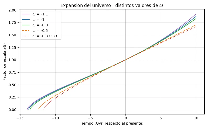
The first reading of Figure 1 is that, for the three values closest to −1, the curves are practically indistinguishable over the whole past range and only begin to separate from t ≈ +3 Gyr. This reflects the very high precision with which Planck constrains ω = −1.03 ± 0.03: close to that value, the past history of the universe is indistinguishable from that of the pure ΛCDM model. In contrast, the curves with ω = −0.5 and ω = −1/3 separate already in the past (they reach a → 0 some 2 Gyr later, which gives lower ages) and, above all, in the future: with ω = −1/3 the expansion is asymptotically linear and the universe never accelerates.

3.2. The distant future and the fate of the universe

To see the role of ω clearly, the integration is extended and a(t) is plotted on a logarithmic scale (Figure 2). On that scale, an exponential expansion appears as a straight line, which makes comparison easier.

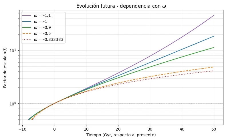
Figure 2 conveys three ideas:

1. For ω = −1 (pure ΛCDM), the scale factor grows exponentially, a(t) ∝ exp(H_∞ · t), with H_∞ = H₀ √Ω_E ≈ 5.7 × 10⁻¹¹ year⁻¹. That expansion leads, over a time of the order of several Hubble times, to a De Sitter universe in which most galaxies leave the horizon and the CMB temperature tends to a very small finite value (Gibbons and Hawking, 1977).
2. For ω = −0.9 (close to −1, although outside Planck’s interval), the expansion keeps accelerating but is no longer exponential: the dark-energy density dilutes slowly and, in the long run, a(t) ∝ t^2/(3(1+ω)) = t^6.7, a very fast power law that on a logarithmic scale gradually bends below the De Sitter straight line.
3. For ω < −1 (the ω = −1.10 curve), the dark-energy density grows with a, which feeds back into the acceleration and produces a runaway: the scale factor diverges in a finite time, the phenomenon known as the Big Rip (Caldwell, Kamionkowski and Weinberg, 2003). Applying those authors’ analytical expression to the parameters of Planck Collaboration (2020) gives a horizon to the singularity of ≈ 117 Gyr, in agreement with the numerical limit at which the integration diverges (t ≈ 116 Gyr; see Figure 3). Before that singularity, gravitationally bound structures become progressively unbound in inverse order of their mean density.

The three regimes are summarised quantitatively in Table 2, together with the present acceleration and the deceleration parameter q₀.

ω adopted	Regime	q₀	ä today (year⁻²)	Fate
−1.10	Phantom energy	−0.630 ± 0.012	+(2.99 ± 0.07) × 10⁻²¹	Big Rip
−1.00	ΛCDM (pure Λ)	−0.527 ± 0.011	+(2.50 ± 0.06) × 10⁻²¹	Asymptotic De Sitter
−0.90	Quintessence	−0.424 ± 0.010	+(2.02 ± 0.06) × 10⁻²¹	Power-law expansion
−0.50	Strong quintessence	−0.013 ± 0.006	+(6.4 ± 2.6) × 10⁻²³	Almost at the boundary
−1/3	Effective curvature	+0.158 ± 0.004	−(7.5 ± 0.2) × 10⁻²²	Perpetual deceleration

Table 2. Summary of the five scenarios analysed. The deceleration parameter was calculated as q₀ = ½Ω_M + Ω_R + ½(1 + 3ω)Ω_E; the present acceleration ä is the direct output of the Friedmann equation at a = 1.

An interesting case: ω = −0.50. The table shows that, for ω = −0.50, the relative error of ä is 40 %, huge compared with the ~2–3 % of the other cases. This is because, close to ω = −1/3, the acceleration passes through zero (it is the boundary between accelerating and decelerating). In that regime, ä is the difference between two comparable quantities, and the errors of each become comparable to the difference itself. It is not a flaw in the calculation, it is physics: something that is almost zero is being measured, so the relative precision degrades.

As a complementary exploration of the asymptotic behaviour, the integration was extended to t = +1.1598 × 10¹¹ years (≈ 116 Gyr), the limit beyond which the numerical calculation is no longer stable. The result (Figure 3) clearly reveals the dramatic asymmetry that the parameter ω imposes on the fate of the universe.

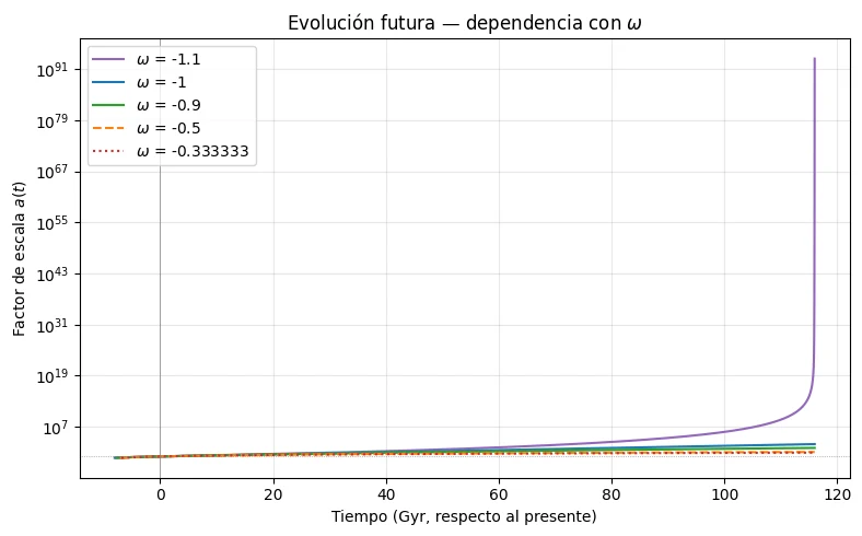
For ω = −0.5 and ω = −1/3, the scale factor barely reaches a ≈ 4 after more than a hundred billion years of expansion, which shows an ever slower sub-exponential regime. For ω = −1, a(t) grows exponentially, consistent with the asymptotic De Sitter solution a(t) ∝ exp(H_∞ t); for ω = −0.9 the growth is almost as fast (power law a ∝ t^6.7), and both exceed a factor of 10² at the end of the interval.

The ω = −1.1 case, on the other hand, shows the unmistakable signature of a finite singularity: the scale factor shoots up to a ~ 10⁹¹ in the last ten gigayears of the simulated range and diverges super-exponentially. The interruption of the integrator with the error OverflowError: Numerical result out of range at t ≈ 1.16 × 10¹¹ years is not an artefact of the Euler scheme but the computational translation of the model’s real singularity: the Big Rip predicted analytically by Caldwell, Kamionkowski and Weinberg (2003), whose characteristic time for ω = −1.1 is estimated at ≈ 117 Gyr.

That the numerical divergence comes slightly before the analytical singularity is to be expected: when the quantities involved (a and its derivative ȧ) grow so fast that some intermediate product exceeds the limit of double-precision floating-point numbers (~10³⁰⁸), the integrator stops. This reinforces the physical reading: small deviations of ω below −1, although indistinguishable on the observational scales accessible today, would condemn the universe to structural disintegration within a finite cosmological horizon.

3.3. Evolution of the densities: the two cosmic transitions

The previous simulations show how the scale factor a(t) evolves under different dark-energy scenarios, but the underlying dynamics (which component dominates at each epoch) remain hidden behind the overall sum. To make this composition explicit, Figure 4 shows the density of each component as a function of the scale factor.

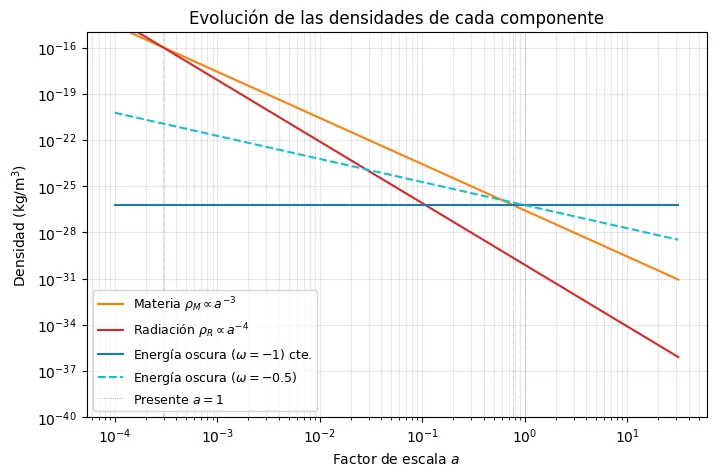
The slopes on the log-log scale are the powers derived in section 1.3: −3 for matter, −4 for radiation, 0 for dark energy with ω = −1 and −3(1 + ω) = −1.5 for ω = −0.5, included as an illustrative contrast. This figure does not come from the numerical integration of the simulations but from directly evaluating the analytical expressions ρ_i(a) = ρ_i,0 · a^−3(1+ω_i) on a logarithmic grid of the scale factor. This makes it possible to identify visually two cosmic transitions of critical physical significance:

• Matter–radiation equality: z_eq,MR = 3402 ± 26 (Planck Collaboration, 2020, Table 2), equivalent to a scale factor a_eq,MR ≈ 2.94 × 10⁻⁴ and to a time t ≈ 51,000 years after the Big Bang. Before that point, radiation dominated the dynamics (red line above the orange one in Figure 4) and photon pressure prevented the gravitational collapse of the primordial inhomogeneities. Afterwards, matter takes control and the regime begins in which the primordial perturbations can grow and give rise to the large-scale structures observed today (Dodelson, 2003).
• Matter–dark energy equality: from Ω_M = 0.3153 ± 0.0073 and Ω_Λ = 0.6847 ± 0.0073 (Planck Collaboration, 2020), imposing ρ_M = ρ_Λ gives a_eq,MΛ = (Ω_M/Ω_Λ)^1/3 = 0.772 ± 0.007, equivalent to a redshift z_eq,MΛ = 0.295 ± 0.012 and to a time in the past of about 3.5 Gyr. To put the time scale in context: at that moment the Earth had already formed and microbial life had been evolving for billions of years. Before that crossing, matter dominated (orange line above the blue one in Figure 4) and the universe decelerated under its own gravitational weight; afterwards, dark energy takes control and the universe enters an accelerating regime. This is therefore the transition that physically explains why we observe an accelerating universe today (Riess et al., 1998; Perlmutter et al., 1999).

The coincidence problem. The matter–Λ crossing took place only the equivalent of 25.4 % of the age of the universe ago, which means that we live in a cosmologically exceptional epoch: the very moment at which the universe changes its dynamical nature. This is the so-called cosmic coincidence problem (Steinhardt, 1997; Zlatev, Wang and Steinhardt, 1999): why do we happen to observe the universe just when its two dominant components, matter and dark energy, have comparable densities, if that coincidence occurs only during a very small fraction of cosmic history? There is no consensus on the answer. One interpretation is the anthropic principle: only in this epoch can observers like us exist, since earlier the structures had not yet formed and later the acceleration will have dispersed the galaxies and the matter will have become too dilute. Another, more physically substantive, is that dark energy is not an inert cosmological constant Λ but a dynamical quintessence-type field whose potential V(φ) converges naturally towards the present regime through tracking dynamics, which would avoid the fine-tuning that Λ requires (Zlatev, Wang and Steinhardt, 1999). The observations of the next two decades, especially those of Euclid and Roman, should decide between the two hypotheses.

4. Discussion and physical interpretation

The results confirm, within the simplified framework of this analysis, the three essential features of the standard cosmological model.

I. There was a Big Bang. For the five values of ω considered, the integration into the past reaches a → 0 in a finite time. The age obtained varies moderately with ω, between about 11.6 Gyr (ω = −1/3) and 14.0 Gyr (ω = −1.1), a spread of about 10 % around the central value. This variation, although visible in Figure 1, is modest because the dynamics of the early universe are dominated by radiation and matter, not by dark energy, which only controls the expansion during the last ≈ 6 Gyr of cosmic history. For the reference case ω = −1, 13.78 ± 0.11 Gyr is obtained, in agreement, within less than 1σ, with the value published by Planck Collaboration (2020) of 13.797 ± 0.023 Gyr.

II. The present expansion is accelerating. In the ΛCDM model, the transition from a decelerating to an accelerating regime (q = 0) takes place at a ≈ 0.61, about 6 Gyr ago, when the matter density falls below twice that of dark energy (ρ_M = 2ρ_Λ). Somewhat later, at a ≈ 0.77 (some 3.5 Gyr ago), strict equality of densities, ρ_M = ρ_Λ, is reached and dark energy becomes the dominant component for good. This result cannot be freely adjusted in the model: it is imposed by the ratio Ω_M/Ω_Λ measured by Planck Collaboration (2020) and is one of the most solid predictions of the ΛCDM model. In the limiting case ω = −1/3, acceleration never occurs (q₀ = +0.158 according to Table 2): the universe would settle into an asymptotically linear expansion, in direct contradiction with the observations of type Ia supernovae that discovered the acceleration (Riess et al., 1998; Perlmutter et al., 1999) and that the ΛCDM model reproduces naturally.

III. The future fate depends critically on ω. For ω = −1 (pure cosmological constant), the universe expands exponentially for ever, distant galaxies leave the horizon and the CMB temperature tends to a very small finite value (Gibbons and Hawking, 1977). For −1 < ω < −1/3 (quintessence), the universe also expands for ever and in an accelerated way, but following a power law instead of an exponential. For ω < −1 (phantom energy), the acceleration runs away and the universe ends in a Big Rip in a finite time; for ω = −1.1, this horizon is ≈ 117 Gyr (section 3.2), in agreement with the analytical solution of Caldwell, Kamionkowski and Weinberg (2003). Measuring ω with the precision needed to distinguish between these fates is the central aim of the Euclid (Euclid Collaboration et al., 2025) and Roman (Spergel et al., 2015) missions, and the DESI results point in that direction: after the first tensions of 2024 (DESI Collaboration, 2024), the second data release (DR2, 2025) prefers a dynamical dark energy (w₀ > −1, w_a < 0) with a significance of 2.8–4.2σ depending on the supernova sample combined (DESI Collaboration, 2025).

Conclusions

The Friedmann acceleration equation has been derived and integrated numerically for a flat universe dominated by matter, radiation and dark energy. With the parameters of Planck Collaboration (2020) in their natural units and propagating their 1σ errors, the model satisfactorily reproduces the fundamental observables of the ΛCDM model: the age of the universe (13.78 ± 0.11 Gyr), the Hubble time (14.51 ± 0.11 Gyr) and the present deceleration parameter (q₀ = −0.527 ± 0.011), all compatible with the published values within less than 1σ.

The systematic exploration of the parameter ω confirms that ω = −1/3 acts as the theoretical boundary between two qualitatively different universes (q₀ > 0 versus q₀ < 0) and that the ultimate fate is controlled by the sign of (ω + 1): eternal expansion for ω ≥ −1 (exponential for ω = −1 and power-law for −1 < ω < −1/3) and a Big Rip for ω < −1. The agreement between the numerical instability horizon (t ≈ 117 Gyr for ω = −1.1) and the time of the singularity predicted analytically by Caldwell, Kamionkowski and Weinberg (2003) is a cross-check of the numerical scheme.

The graphical identification of the two cosmic transitions (matter–radiation equality at a ≈ 2.94 × 10⁻⁴ and matter–dark energy equality at a ≈ 0.77) puts the present epoch in context: the latter of these transitions happened only 3.5 Gyr ago, 25 % of the total age of the universe. The accelerating regime proper (q < 0) began somewhat earlier, at a ≈ 0.61 (≈ 6 Gyr ago). Living so close to the moment when the universe changes its dynamical nature is the cosmic coincidence problem (Zlatev, Wang and Steinhardt, 1999), one of the observational arguments that motivate the exploration of alternatives to the cosmological constant, such as dynamical quintessence, whose resolution will fall to the next generations of cosmological observatories.

Appendix. Tools used

This appendix describes the computational tools used to produce the numerical results and the figures. The whole development is contained in a Jupyter notebook.

A.1. Environment and dependencies. The analysis was carried out entirely in Python 3 in a Jupyter notebook. The only dependencies are three libraries of the standard scientific ecosystem: math (standard module), for mathematical constants such as π; NumPy (Harris et al., 2020), for handling arrays and vectorised operations; and Matplotlib (Hunter, 2007), for all the figures. No specialised cosmological libraries were used, deliberately, because of the aim of the work: to build the model from first principles.

A.2. Numerical integration scheme. The Friedmann acceleration equation d²a/dt² = f(a, ω) is integrated with a first-order explicit Euler scheme, rewriting the second-order ordinary differential equation as a system of two first-order equations with the auxiliary variable v ≡ da/dt. In each iteration of the while loop, the velocity is first updated with the instantaneous acceleration and then the scale factor with the newly calculated velocity. The time step Δt = 10⁷ years is 1/1450 of the Hubble time, small enough for the global Euler error to stay below 0.1 % over the whole range. Integration into the past is obtained by reversing the sign of the step. The stopping conditions are a = 0.01 towards the past and t = 10¹⁰ years towards the future in the standard simulations; t = 5 × 10¹⁰ years and t = 1.1598 × 10¹¹ years in the extended-future analyses.

A.3. Organisation of the notebook and workflow. The notebook is organised in three functional blocks:

1. Block 1: constants and original integration loops. Cells in which the numerical values of H₀, G, ρ_M,0, ρ_R,0 and ρ_E,0 are assigned, and the original while loops of the base notebook (one for the past and one for the future), which produce the individual simulation for a single value of ω and its basic plot.
2. Block 2: reusable function and systematic sweep over ω. To avoid repeating the code five times, the loops of block 1 are wrapped in the function simular(omega, t_futuro_max, a_pasado_min), which returns an (N, 2) array with the time in Gyr and the scale factor. From it, the list omegas = [−1.10, −1.00, −0.90, −0.50, −1/3] is iterated to produce the five curves of Figure 1 and, by increasing t_futuro_max, Figure 2.
3. Block 3: checks and complementary figures. It includes the calculation of derived quantities (age of the universe, q₀ and present acceleration for each ω); the convergence check of the Euler scheme, calculating the age with five time steps between 10⁶ and 2 × 10⁷ years and checking that the figures agree to within 0.01 Gyr; the exploration of the Big Rip through an integration extended to t = 1.1598 × 10¹¹ years for ω = −1.1; and the evaluation of the analytical densities ρ_i(a) on a logarithmic grid, which generates Figure 4.

A.4. Reproducibility. The whole analysis is reproducible by running the notebook cells in sequence. The intermediate results of each simulation are saved automatically to text files with the pattern expansionUniverso_<omega>.txt. No random seed is required, because the integration is completely deterministic, and the full calculation takes less than a minute on a standard computer.

References

• Caldwell, R. R., Kamionkowski, M., & Weinberg, N. N. (2003). Phantom energy: Dark energy with w < −1 causes a cosmic doomsday. Physical Review Letters, 91(7), 071301.
• DESI Collaboration (2024). DESI 2024 VI: Cosmological constraints from the measurements of baryon acoustic oscillations. arXiv:2404.03002.
• DESI Collaboration (2025). DESI DR2 results II: Measurements of baryon acoustic oscillations and cosmological constraints. arXiv:2503.14738.
• Dodelson, S. (2003). Modern Cosmology. Academic Press.
• Euclid Collaboration, Mellier, Y., et al. (2025). Euclid. I. Overview of the Euclid mission. Astronomy & Astrophysics, 697, A1.
• Friedmann, A. (1922). Über die Krümmung des Raumes. Zeitschrift für Physik, 10(1), 377–386.
• Gibbons, G. W., & Hawking, S. W. (1977). Cosmological event horizons, thermodynamics, and particle creation. Physical Review D, 15(10), 2738–2751.
• Harris, C. R., Millman, K. J., van der Walt, S. J., et al. (2020). Array programming with NumPy. Nature, 585, 357–362.
• Hogg, D. W. (1999). Distance measures in cosmology. arXiv:astro-ph/9905116.
• Hubble, E. (1929). A relation between distance and radial velocity among extra-galactic nebulae. Proceedings of the National Academy of Sciences, 15(3), 168–173.
• Hunter, J. D. (2007). Matplotlib: A 2D graphics environment. Computing in Science & Engineering, 9(3), 90–95.
• Lemaître, G. (1927). Un univers homogène de masse constante et de rayon croissant rendant compte de la vitesse radiale des nébuleuses extra-galactiques. Annales de la Société Scientifique de Bruxelles, A47, 49–59.
• Penzias, A. A., & Wilson, R. W. (1965). A measurement of excess antenna temperature at 4080 Mc/s. The Astrophysical Journal, 142, 419–421.
• Perlmutter, S., et al. (1999). Measurements of Ω and Λ from 42 high-redshift supernovae. The Astrophysical Journal, 517(2), 565–586.
• Planck Collaboration (2020). Planck 2018 results. VI. Cosmological parameters. Astronomy & Astrophysics, 641, A6.
• Riess, A. G., et al. (1998). Observational evidence from supernovae for an accelerating universe and a cosmological constant. The Astronomical Journal, 116(3), 1009–1038.
• Spergel, D., et al. (2015). Wide-Field InfrarRed Survey Telescope-Astrophysics Focused Telescope Assets WFIRST-AFTA 2015 report. arXiv:1503.03757.
• Steinhardt, P. J. (1997). Cosmological challenges for the 21st century. In V. L. Fitch, D. R. Marlow and M. A. E. Dementi (Eds.), Critical Problems in Physics (pp. 123–147). Princeton University Press.
• Tiesinga, E., Mohr, P. J., Newell, D. B., & Taylor, B. N. (2021). CODATA recommended values of the fundamental physical constants: 2018. Reviews of Modern Physics, 93(2), 025010.
• Zlatev, I., Wang, L., & Steinhardt, P. J. (1999). Quintessence, cosmic coincidence, and the cosmological constant. Physical Review Letters, 82(5), 896–899.