Stellar astrophysics · UNIR
Analysis of pulsating stars: a δ Scuti observed by Kepler
Fourier transform and prewhitening with Period04 on a Kepler light curve: identification of the significant frequencies, multi-frequency fit, rejection of the satellite’s spurious frequencies and classification of the pulsator type following Aerts et al. (2010).

Introduction
Stars are not static objects: some show periodic variations in brightness caused by internal oscillations that change their density, pressure and temperature. These are the pulsating stars, whose study makes it possible to infer their internal structure, something that cannot be observed directly.
This work analyses radial pulsations, those in which the star expands and contracts while keeping its spherical symmetry. These oscillations are driven by the κ mechanism, a process that takes place in partially ionised layers and acts like a heat engine: during contraction the opacity increases and the layer traps energy; during expansion the opacity decreases and the energy is released, producing the observed changes in luminosity.
Asteroseismology studies these brightness variations in the same way that seismology analyses the vibrations of the Earth. Thanks to missions such as Kepler, high-precision light curves are available that make it possible to identify pulsation modes. In this report, the Fourier transform is applied with Period04 to detect the significant frequencies, perform a multi-frequency fit and, finally, propose the pulsation type following Aerts’s classifications.
Exercise 1. Identification of the first significant frequency
From a time series of real data observed by the Kepler satellite, the first significant frequency is sought, its amplitude, phase and signal-to-noise ratio (SNR) are determined, and the amplitude spectrum is plotted.
Any signal that changes with time, including the light curve of a star, can be decomposed as the sum of many sine waves (Aerts, Christensen-Dalsgaard and Kurtz, 2010), that is, waves of the form:
A · sin(2π f t + φ)
where:
- A is the amplitude (how strongly it oscillates).
- f is the frequency (how many times it oscillates per day).
- φ is the phase (where in the cycle the wave is when the measurement starts).
In this way, however complex, irregular or noisy the signal may look, it can be analysed as a mixture of simple waves. To do so, the Fourier transform is first applied to the original light curve, giving the amplitude spectrum: the decomposition of the star’s brightness variability into its sinusoidal components.
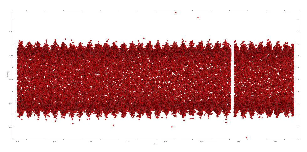
Figure 1 shows the flux variation observed by Kepler over almost 30 days. A clearly detectable periodic modulation can be seen, superimposed on instrumental noise and on a gap in the data associated with the acquisition pauses typical of the mission.
To identify the first significant frequency, a sequential process is followed, starting with the calculation of the amplitude spectrum of the original data.
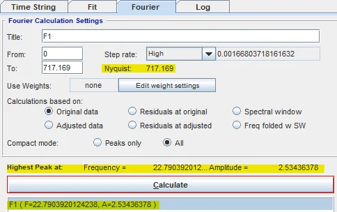
Spectrum calculation. The amplitude spectrum of the original time series is calculated within the range allowed by the sampling. In these data, the Nyquist frequency, the highest that can be detected unambiguously, is 717.169 d⁻¹. From this spectrum the dominant peak, which corresponds to the first significant frequency, is identified.
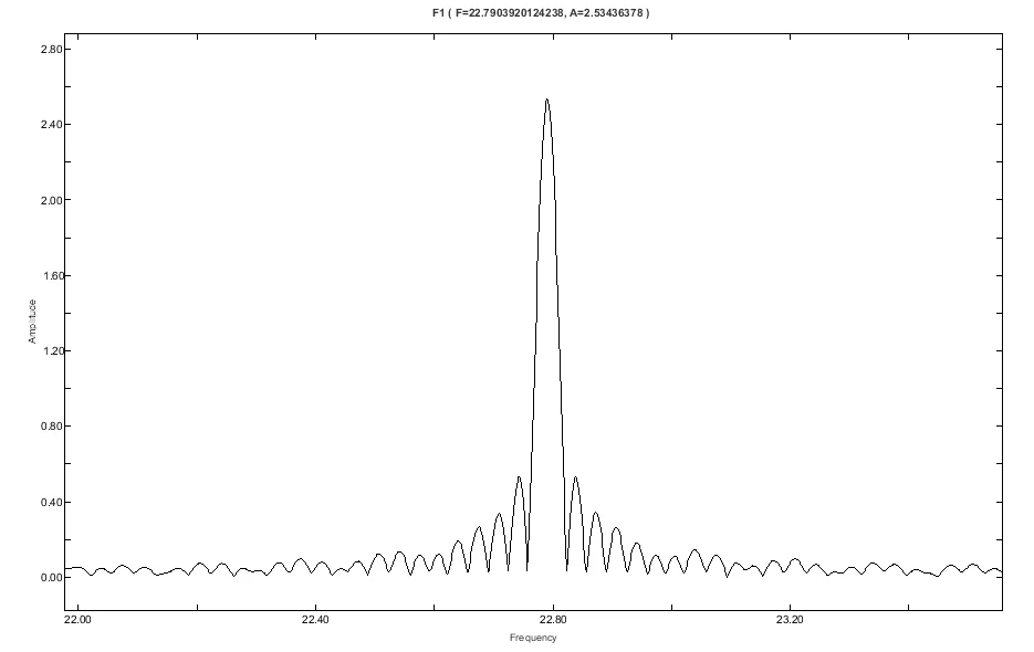
Identification. The frequency with the highest amplitude is f₁ = 22.790 d⁻¹, which represents the dominant oscillation mode of the star. In the amplitude spectrum (Figure 3), each peak represents a sinusoidal oscillation present in the light curve, and its height corresponds to the amplitude of that oscillation (A = 2.534 mmag).
Conceptually, identifying the first frequency means detecting the oscillation mode that contributes most energy to the observed brightness. Besides the central maximum, other lower-amplitude peaks are found throughout the spectrum that exceed the significance threshold used (SNR ≥ 4); these are discussed later. This indicates that, although most of the variability is concentrated in the dominant frequency, the star has multiple oscillation modes that also contribute to the observed signal.
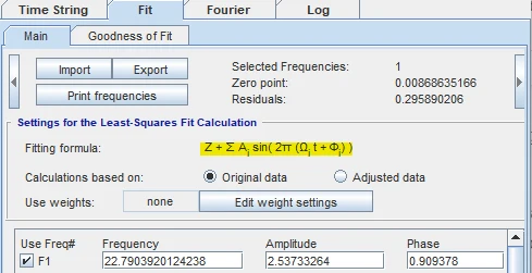
Fit. The frequency, amplitude and phase are fitted simultaneously by non-linear least squares, in order to obtain the most precise values and be able to reconstruct the light curve.
Significance. Before looking for a new frequency, the SNR of the frequency just identified must be calculated. This calculation is not done on the original data but on the residuals, that is, on the light curve from which the fitted frequency has already been subtracted.
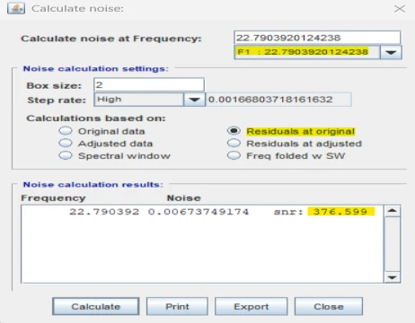
Following the standard criterion for Kepler photometric data, a frequency is considered significant only if SNR ≥ 4. The very high signal-to-noise ratio obtained, SNR = 376.599, indicates that this mode is physically real and dominates the variability of the star; in a pulsating star it usually corresponds to a radial or dominant mode. Table 1 lists the fundamental parameters of this frequency.
| Parameter | Value | Unit |
|---|---|---|
| Frequency (f₁) | 22.790 | cycles/day (d⁻¹) |
| Amplitude (A₁) | 2.533 | mmag |
| Phase (φ₁) | 0.909 | fraction of cycle |
| Signal-to-noise ratio (SNR₁) | 376.599 | — |
Table 1. Fitted parameters of the first frequency f₁ (dominant mode).
These values summarise the key information of the process: the position of the most prominent peak in the frequency domain, its photometric amplitude, the phase that defines the time offset of the signal and the high signal-to-noise ratio that confirms its physical nature. They complete the characterisation of the main mode, which is responsible for most of the variability of the light curve.
Exercise 2. Analysis of the second significant frequency
Since the first frequency comfortably exceeds the significance criterion, the process is repeated for the second significant frequency, determining its amplitude, phase and SNR, and its spectrum is compared with the previous one.
The general dynamics of the method are the same, but from this point on the Fourier transform is no longer calculated on the original data but on the residuals. This reveals the peaks that were partly hidden beneath the power of the main mode.
| Parameter | Value | Unit |
|---|---|---|
| Frequency (f₂) | 21.714 | cycles/day (d⁻¹) |
| Amplitude (A₂) | 0.250 | mmag |
| Phase (φ₂) | 0.284 | fraction of cycle |
| Signal-to-noise ratio (SNR₂) | 73.108 | — |
Table 2. Fitted parameters of the second frequency.
The second significant frequency has a considerably lower amplitude than the dominant one, but its high SNR confirms that it is a real oscillation mode.
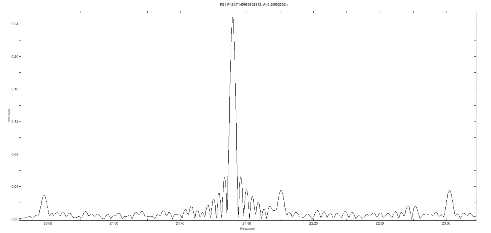
With the main mode removed beforehand, this second peak becomes clearly visible in the spectrum of the residuals, where it becomes the new most prominent signal. A narrow, well-defined peak appears at 21.714 d⁻¹, with an overall power level noticeably lower than before, and secondary peaks appear that were previously partly masked by the amplitude of f₁. This behaviour is what is expected in a prewhitening process: each successive subtraction cleans the spectrum and makes weaker modes easier to detect.
The two spectra studied therefore have their own characteristics:
- Change in the amplitude scale. The spectrum of the second frequency has much smaller amplitude values than that of f₁.
- Greater relative visibility of the secondary peaks. Signals that were partly hidden beneath the power of the main mode now emerge clearly.
- New dominant peak. The frequency f₂ = 21.714 d⁻¹ becomes the maximum of the spectrum, something that could not be seen before because of the absolute dominance of the first mode.
These differences confirm that the procedure is correct: by removing each significant mode, the residual spectrum reveals the real multi-periodic structure of the star.
Exercise 3. Detection of the full set of frequencies
Next, all the other frequencies of the star are determined following the significance criterion SNR ≥ 4. The procedure is repeated systematically: apply a new Fourier transform to the residuals, fit the frequency detected, calculate its SNR and check whether it exceeds the threshold. This iterative process progressively reveals all the oscillation modes present in the star, and it stops when SNR < 4.
The criterion SNR ≥ 4 (Breger et al., 1993; Aerts et al., 2010) is the standard in high-precision photometry for deciding whether a peak in the Fourier spectrum corresponds to a real oscillation of the star or is simply a statistical fluctuation of the noise.
| Iteration | Frequency (d⁻¹) | Amplitude (mmag) | Phase | Noise (mmag) | SNR |
|---|---|---|---|---|---|
| F1 | 22.7904 | 2.5327 | 0.9094 | 0.0067 | 376.5990 |
| F2 | 21.7145 | 0.2503 | 0.2844 | 0.0034 | 73.1078 |
| F3 | 23.0222 | 0.0384 | 0.7307 | 0.0031 | 12.2776 |
| F4 | 20.5752 | 0.0317 | 0.9335 | 0.0018 | 17.7458 |
| F5 | 0.0534 | 0.0286 | 0.7511 | 0.0030 | 8.9366 |
| F6 | 22.0148 | 0.0302 | 0.8581 | 0.0032 | 8.5519 |
| F7 | 21.9647 | 0.0247 | 0.4722 | 0.0026 | 9.4226 |
| F8 | 42.5917 | 0.0219 | 0.5318 | 0.0022 | 9.8152 |
| F9 | 22.8137 | 0.0180 | 0.5764 | 0.0023 | 9.4848 |
| F10 | 10.3285 | 0.0139 | 0.2907 | 0.0021 | 6.5611 |
| F11 | 22.7620 | 0.0129 | 0.8319 | 0.0020 | 6.6163 |
| F12 | 11.9982 | 0.0111 | 0.0240 | 0.0020 | 5.4162 |
| F13 | 0.3319 | 0.0110 | 0.1559 | 0.0026 | 4.1530 |
| F14 | 43.5975 | 0.0107 | 0.5519 | 0.0020 | 5.2529 |
| F15 | 0.1101 | 0.0096 | 0.8080 | 0.0024 | 4.0391 |
| F16 | 42.2797 | 0.0089 | 0.2416 | 0.0018 | 4.8291 |
| F17 | 9.9015 | 0.0086 | 0.9808 | 0.0020 | 4.4897 |
| F18 | 43.3690 | 0.0087 | 0.6921 | 0.0019 | 4.6758 |
| F19 | 9.4878 | 0.0084 | 0.9800 | 0.0018 | 4.5506 |
| F20 | 679.5884 | 0.0083 | 0.6932 | 0.0020 | 4.2288 |
| F21 | 326.5817 | 0.0078 | 0.2204 | 0.0019 | 3.9897 |
Table 3. Frequencies obtained with the iterative prewhitening process, with their amplitudes, phases and signal-to-noise ratios.
This table is the final result of the prewhitening process: every frequency with SNR ≥ 4 was identified, fitted and subtracted from the data set, which revealed ever weaker modes. The last significant frequency appears at iteration 21, which marks the end of the process.
Exercise 4. Global fit of the light curve
With all the frequencies validated, the light curve is fitted with all the significant frequencies at once, reconstructing the observed signal by combining all the detected modes simultaneously. In this way, the final model includes only the physical oscillations of the star and excludes the residual noise.
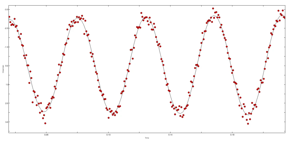
The overlay of the model on the data shows an almost perfect match. This confirms that the modes extracted during prewhitening faithfully reproduce the periodic variability of the star and that no further frequencies are needed to describe its pulsating behaviour.
In addition, the fit makes it possible to extrapolate the star’s behaviour into intervals without measurements caused by gaps in data acquisition. Figure 8 shows a clear example: although the time series has a break, the model continuously reproduces the variability expected from the identified pulsation modes. This is possible because the fit combines all the significant frequencies, so the resulting signal is fully defined even where observations are missing.
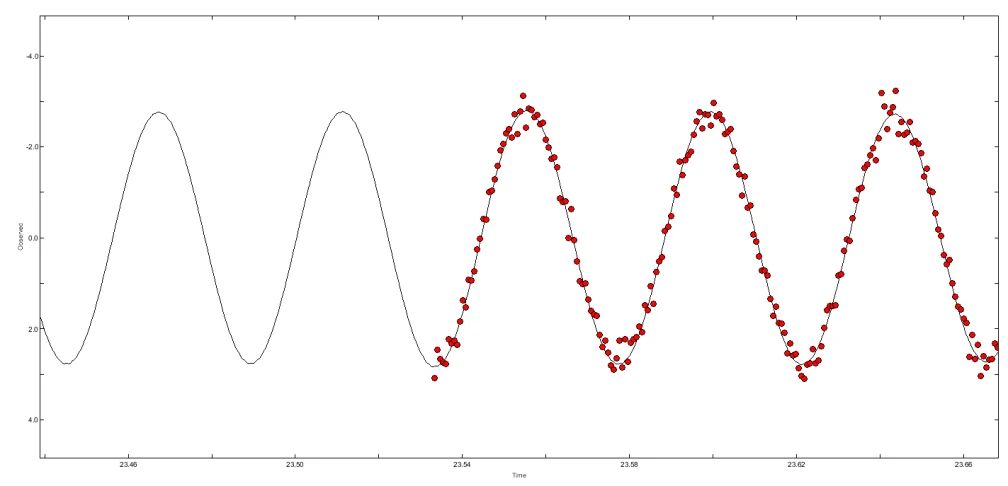
Finally, the small scatter around the fit is due to the photometric noise level of the observations, not to the presence of additional oscillations.
Exercise 5. Rejection of spurious frequencies and mode identification
To select the most representative frequencies of the star and reject the spurious frequencies of the Kepler satellite, the frequency column of Table 3 was compared with the list of short-cadence spurious frequencies published for the mission (SC spurious frequency summary; Christiansen et al., 2016). The comparison looked for numerical matches within the width given as narrow or broad in that table. The following was found:
- Real modes. None of the frequencies in the range ~20 to 23 d⁻¹ (F1, F2, F3, F4, F6, F7, F9 and F11) matches the typical spurious lines of the satellite (7.50; 16.98; 20.95; 25.06; 29.38; 31–32 d⁻¹, etc.), so they can be considered real pulsation modes. F4 lies near a region contaminated by the satellite, but it does not match the listed instrumental frequency, so it is treated as a pulsation mode.
- Doubtful frequencies. The low frequencies F5, F13 and F15 (≈ 0.05–0.33 d⁻¹) do not appear in the artefact table but, being close to 0 d⁻¹, they are candidates for long-term trends or instrumental effects, and they are flagged as doubtful.
- Instrumental frequency. The very high frequency F20 = 679.59 d⁻¹ falls in the same range as Kepler’s spurious line U7 (~679.54 d⁻¹).
| Iteration | Frequency (d⁻¹) | Amplitude (mmag) | Phase | Noise (mmag) | SNR |
|---|---|---|---|---|---|
| F20 | 679.5884 | 0.0083 | 0.6932 | 0.0020 | 4.2288 |
Table 4. Fitted parameters of frequency F20 and its signal-to-noise ratio, compared with the spurious frequency U7 of the Kepler satellite (Christiansen et al., 2016).
It can therefore be concluded that F20 = 679.588 d⁻¹ is an instrumental frequency, associated with the satellite’s sampling, and it is rejected as a pulsation mode of the star. F21 had already been rejected for not meeting the criterion SNR ≥ 4.
To determine what type of star is being observed, the representative frequencies are compared with the tables of Aerts et al. (2010), and the possible pulsation types are discussed. In asteroseismology, when a frequency is expressed in cycles per day (d⁻¹), the period is obtained simply as:
P = 1 / f
where P is the period (in days) and f the frequency (in cycles per day). Taking f₁ = 22.790 d⁻¹ gives P = 0.0438 days; multiplying by 24, P = 1.0526 h.
Extending this calculation to all the frequencies that were not rejected, groups can be formed according to their period and the mean pulsation period of each can be calculated in hours, to finally propose which type of star is most compatible according to the table of Aerts, Christensen-Dalsgaard and Kurtz (2010):
| Group | Frequency (d⁻¹) | Iterations | Mean period (h) | Compatibility (Aerts) |
|---|---|---|---|---|
| I | 20 – 23 | F1, F2, F3, F4, F6, F7, F9, F11 | 1.0821 | δ Sct |
| II | 42 – 43 | F8, F14, F16, F18 | 0.5588 | δ Sct, g-mode sdBV?, GW Vir? |
| III | 9 – 12 | F10, F12, F17, F19 | 2.3194 | δ Sct, β Cep?, pulsating T Tauri?, pulsating Herbig Ae/Be? |
Table 5. Grouping of the representative frequencies and comparison of the mean periods with the typical pulsation ranges according to Aerts et al. (2010).
The detected modes have periods between about 0.5 and 3 hours, which falls squarely in the characteristic range of δ Scuti stars, whose typical periods range from 15 minutes to 8 hours (Aerts et al., 2010). This behaviour corresponds to pressure modes (p modes), consistent with the fast, high-frequency oscillations shown by the spectrum.
In addition, the amplitudes obtained (between ~2.53 mmag and ~0.008 mmag) are also compatible with δ Scuti stars, which show light variations well below 0.3 mag (300 mmag). Both the periods and the amplitudes therefore place the star within the typical regime of this class.
Comparing the observed periods with the other families in Aerts’s table reveals some partial matches. These other families can, however, be ruled out: although some have period ranges that partly overlap with the observed values, they have physical properties incompatible with the signal analysed. For example, β Cep stars have typical periods of about 2 to 8 h (Stankov and Handler, 2005; Aerts et al., 2010), which matches only group III; groups I and II, which are faster, lie below their lower limit. β Cep cannot explain the shortest periods, and only a δ Scuti star reproduces all three groups simultaneously.
In summary, the periods, the amplitudes, the number of modes detected and the structure of the spectrum consistently match a δ Scuti star. The other candidates appear as partial matches in one group or another, but they cannot reproduce the whole observed pulsation pattern. This classification is the one that best fits the set of properties derived from the asteroseismic analysis.
Conclusion
In this work, 20 significant frequencies (SNR ≥ 4) were identified in the light curve observed by Kepler, 16 of which correspond to reliable pulsation modes (F20 is instrumental and F5, F13 and F15 remain doubtful), after applying an iterative prewhitening analysis and a precise multi-frequency fit. The comparison with the catalogue of instrumental artefacts made it possible to reject the spurious lines and isolate only the real modes of the star. By converting frequencies into periods and comparing them with the classification tables of Aerts et al. (2010), it was determined that all the values obtained lie within the typical pulsation range of δ Scuti stars. The ultra-low amplitudes measured, together with the richness of modes and the final structure of the spectrum, reinforce this classification. The asteroseismic analysis therefore confirms that the star studied is a clear example of a low-amplitude δ Scuti pulsator observed with the photometric precision of the Kepler satellite.
References
- Aerts, C., Christensen-Dalsgaard, J., & Kurtz, D. W. (2010). Asteroseismology. Springer.
- Bracewell, R. N. (1986). The Fourier Transform and Its Applications. McGraw-Hill.
- Breger, M., Stich, J., Garrido, R., et al. (1993). Nonradial pulsation of the delta Scuti star BU Cancri in the Praesepe cluster. Astronomy & Astrophysics, 271, 482–486.
- Christiansen, J. L., Van Cleve, J. E., Jenkins, J. M., Caldwell, D. A., Barclay, T., Bryson, S. T., et al. (2016). Kepler Data Characteristics Handbook (KSCI-19040-005). NASA Ames Research Center; Space Telescope Science Institute.
- Lenz, P., & Breger, M. (2005). Period04 User Guide: An analysis tool for astronomical time series. Communications in Asteroseismology, 146, 53–136.
- NASA Kepler Mission (2013). Photometry data archive. Teaching material for the course Stellar and Interstellar Structure and Evolution, Universidad Internacional de La Rioja.
- Stankov, A., & Handler, G. (2005). Catalog of Galactic β Cephei stars. The Astrophysical Journal Supplement Series, 158(2), 193–216.